Process and integrate data with Seurat and Harmony
Florian Wuenenmann
Last updated: 2022-04-19
Checks: 7 0
Knit directory: Abatacept_scrnaseq_mi/
This reproducible R Markdown analysis was created with workflowr (version 1.7.0). The Checks tab describes the reproducibility checks that were applied when the results were created. The Past versions tab lists the development history.
Great! Since the R Markdown file has been committed to the Git repository, you know the exact version of the code that produced these results.
Great job! The global environment was empty. Objects defined in the global environment can affect the analysis in your R Markdown file in unknown ways. For reproduciblity it’s best to always run the code in an empty environment.
The command set.seed(20220318) was run prior to running the code in the R Markdown file. Setting a seed ensures that any results that rely on randomness, e.g. subsampling or permutations, are reproducible.
Great job! Recording the operating system, R version, and package versions is critical for reproducibility.
Nice! There were no cached chunks for this analysis, so you can be confident that you successfully produced the results during this run.
Great job! Using relative paths to the files within your workflowr project makes it easier to run your code on other machines.
Great! You are using Git for version control. Tracking code development and connecting the code version to the results is critical for reproducibility.
The results in this page were generated with repository version 6fc473c. See the Past versions tab to see a history of the changes made to the R Markdown and HTML files.
Note that you need to be careful to ensure that all relevant files for the analysis have been committed to Git prior to generating the results (you can use wflow_publish or wflow_git_commit). workflowr only checks the R Markdown file, but you know if there are other scripts or data files that it depends on. Below is the status of the Git repository when the results were generated:
Ignored files:
    Ignored:    .Rhistory
    Ignored:    .Rproj.user/

Untracked files:
    Untracked:  code/utils.R
    Untracked:  code/utils_nichenet.R
    Untracked:  data/Table_1_Common Transcriptomic Effects of Abatacept and Other DMARDs on Rheumatoid Arthritis Synovial Tissue.xlsx
    Untracked:  omnipathr-log/

Unstaged changes:
    Deleted:    analysis/7_Conclusions.Rmd
    Deleted:    analysis/7_summary.Rmd
Note that any generated files, e.g. HTML, png, CSS, etc., are not included in this status report because it is ok for generated content to have uncommitted changes.
These are the previous versions of the repository in which changes were made to the R Markdown (analysis/1_process_and_integrate_Seurat_Harmony.Rmd) and HTML (docs/1_process_and_integrate_Seurat_Harmony.html) files. If you’ve configured a remote Git repository (see ?wflow_git_remote), click on the hyperlinks in the table below to view the files as they were in that past version.
| File | Version | Author | Date | Message |
|---|---|---|---|---|
| html | a71b19c | Florian Wuennemann | 2022-04-19 | Build site. |
| html | f472db4 | Florian Wuennemann | 2022-04-14 | Build site. |
| html | 6e3bb2f | Florian Wuennemann | 2022-03-25 | Build site. |
| html | 51698db | Florian Wuennemann | 2022-03-24 | Build site. |
| Rmd | 0ca9e0c | Florian Wuennemann | 2022-03-24 | wflow_publish("analysis/1_process_and_integrate_Seurat_Harmony.Rmd") |
| html | 9cb1481 | Florian Wuennemann | 2022-03-24 | Build site. |
| Rmd | cef1b92 | Florian Wuennemann | 2022-03-24 | wflow_publish("analysis/1_process_and_integrate_Seurat_Harmony.Rmd") |
| html | c0caa6c | Florian Wuennemann | 2022-03-24 | Build site. |
| Rmd | 828b48a | Florian Wuennemann | 2022-03-24 | wflow_publish("analysis/1_process_and_integrate_Seurat_Harmony.Rmd") |
| html | c623d58 | Florian Wuennemann | 2022-03-24 | Build site. |
| Rmd | 9b8eed0 | Florian Wuennemann | 2022-03-24 | wflow_publish("analysis/1_process_and_integrate_Seurat_Harmony.Rmd") |
| html | 29960c2 | Florian Wuennemann | 2022-03-24 | Build site. |
| Rmd | 9ffd61b | Florian Wuennemann | 2022-03-24 | wflow_publish("analysis/1_process_and_integrate_Seurat_Harmony.Rmd") |
| html | b47d7b0 | Florian Wuennemann | 2022-03-24 | Build site. |
| Rmd | 8591656 | Florian Wuennemann | 2022-03-24 | wflow_publish(c("analysis/1_process_and_integrate_Seurat_Harmony.Rmd", |
| html | 46f2db7 | Florian Wuennemann | 2022-03-23 | First commit. |
Aim
Here we will read in the raw 10x Genomics data, process it with Seurat and integrate the control and treatment samples using Harmony.
Read raw data
First, we will read in the raw H5 data using Seurat.
c1 <- Read10X_h5("../raw_data/C1/filtered_feature_bc_matrix.h5")
c1_seurat <- CreateSeuratObject(counts = c1, project = "C1", min.cells =3, min.features = 20)
c2  <- Read10X_h5("../raw_data/C2/filtered_feature_bc_matrix.h5")
c2_seurat <- CreateSeuratObject(counts = c2, project = "C2", min.cells =3, min.features = 20)
i3  <- Read10X_h5("../raw_data/I3/filtered_feature_bc_matrix.h5")
i3_seurat <- CreateSeuratObject(counts = i3, project = "I3", min.cells =3, min.features = 20)
i4  <- Read10X_h5("../raw_data/I4/filtered_feature_bc_matrix.h5")
i4_seurat <- CreateSeuratObject(counts = i4, project = "I4", min.cells =3, min.features = 20)

## add metadata
c1_seurat$group <- "treatment"
c2_seurat$group <- "treatment"
i3_seurat$group <- "control"
i4_seurat$group <- "control"

seurat_object <- merge(c1_seurat, y = c(c2_seurat, i3_seurat,i4_seurat), add.cell.ids = c("C1","C2","CI3", "CI4"), project = "abatacept MI")
Filter data
After reading in the data, we will filter out low quality cells. First let`s look at the raw data distributions and then decide on reasonable thresholds.
Basic QC
First let’s look at some basic QC parameter distributions. We will filter based on some of these paremeters later.
seurat_object[["percent.mt"]] <- PercentageFeatureSet(object = seurat_object, pattern = "^mt-")
VlnPlot(seurat_object, features = c("nFeature_RNA", "nCount_RNA", "percent.mt"), ncol = 3)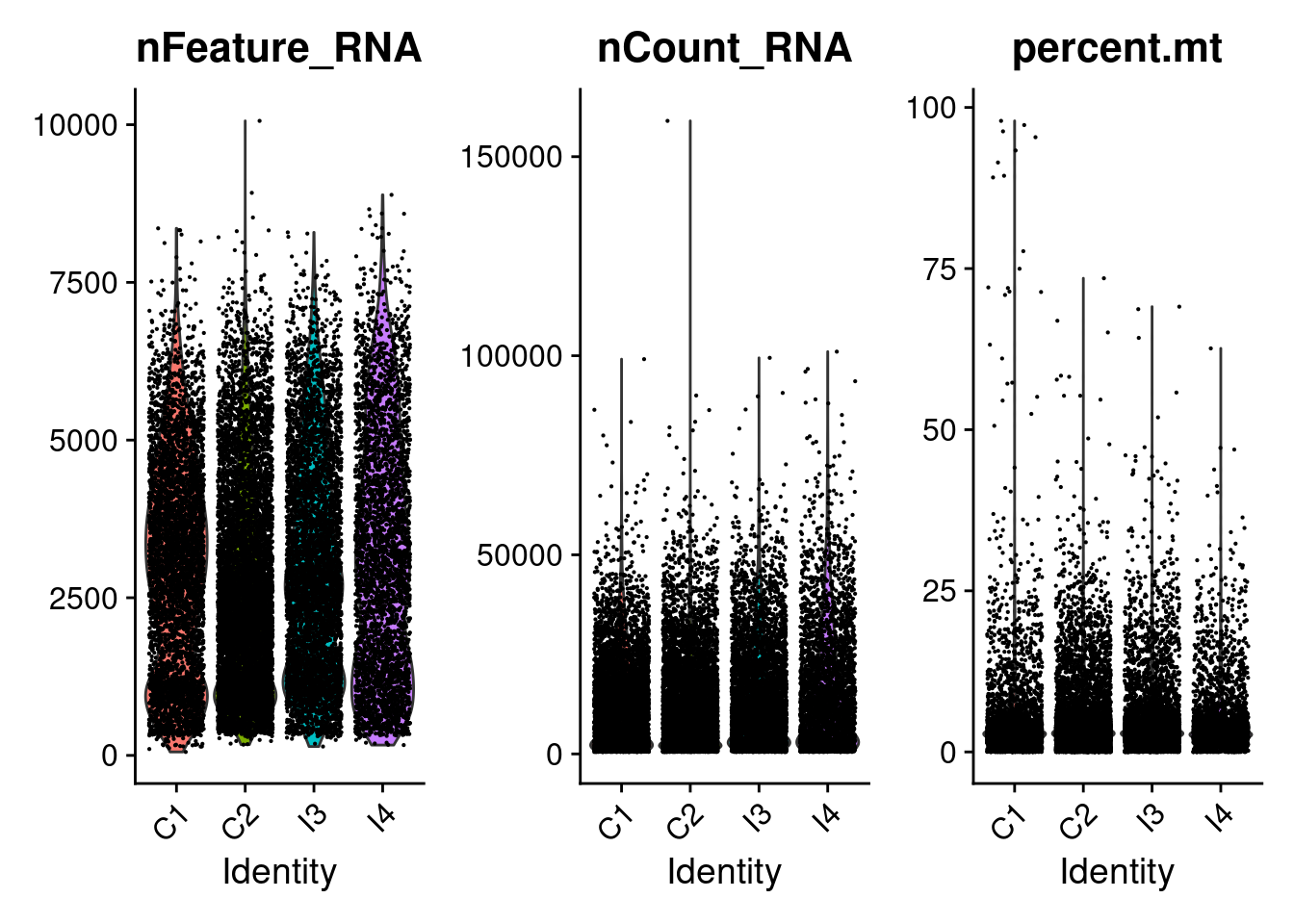
| Version | Author | Date |
|---|---|---|
| b47d7b0 | Florian Wuennemann | 2022-03-24 |
FeatureScatter(seurat_object, feature1 = "nCount_RNA", feature2 = "nFeature_RNA")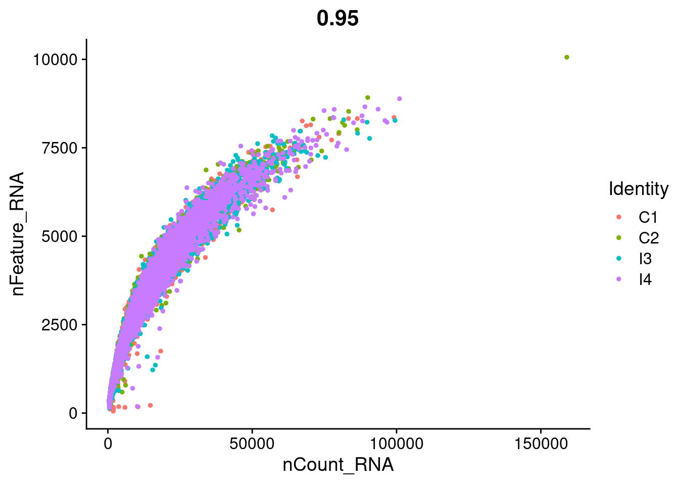
| Version | Author | Date |
|---|---|---|
| b47d7b0 | Florian Wuennemann | 2022-03-24 |
FeatureScatter(seurat_object, feature1 = "nFeature_RNA", feature2 = "percent.mt")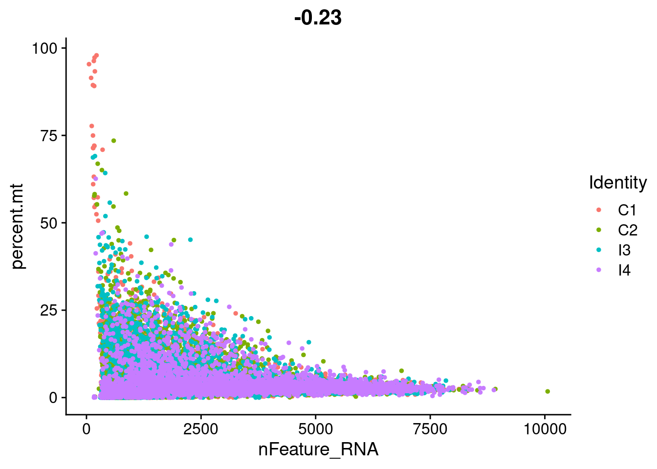
| Version | Author | Date |
|---|---|---|
| b47d7b0 | Florian Wuennemann | 2022-03-24 |
miQC
To identify low-quality cells based on the mitochondrial content of cells we are gonna use the miQC approach by Hippen et al (https://journals.plos.org/ploscompbiol/article?id=10.1371/journal.pcbi.1009290).
Here is a vignette on how to run miQC with Seurat objects: https://htmlpreview.github.io/?https://github.com/satijalab/seurat-wrappers/blob/master/docs/miQC.html
seurat_object <- RunMiQC(seurat_object, percent.mt = "percent.mt", nFeature_RNA = "nFeature_RNA", posterior.cutoff = 0.75,
    model.slot = "flexmix_model")
## Explore parameters fro MiQC
flexmix::parameters(Misc(seurat_object, "flexmix_model")) Comp.1 Comp.2
coef.(Intercept) 2.0205390714 17.869575527
coef.nFeature_RNA 0.0002068304 -0.003027076
sigma 1.3681079842 8.477597350PlotMiQC(seurat_object, color.by = "miQC.probability") + ggplot2::scale_color_gradient(low = "grey", high = "purple")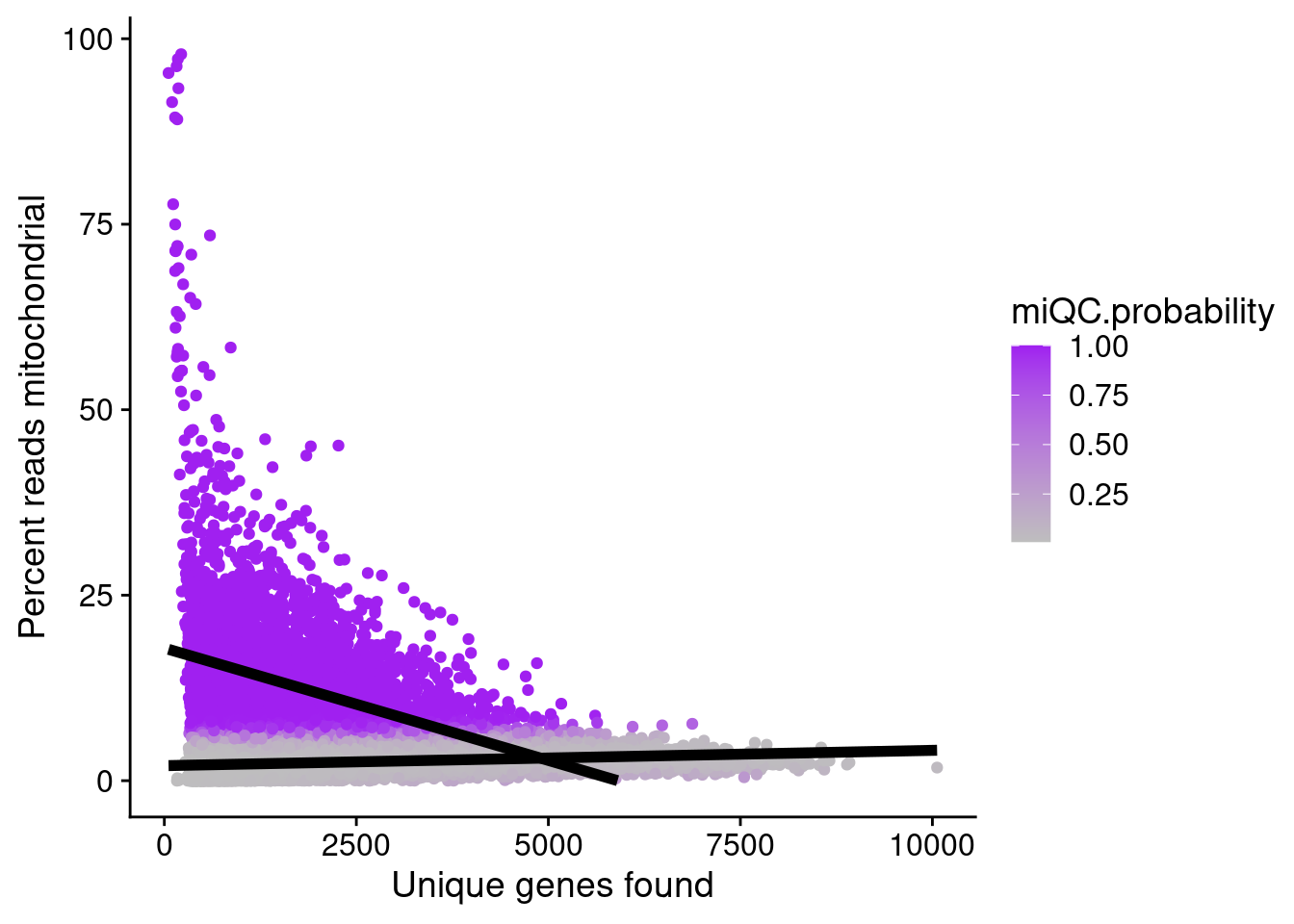
| Version | Author | Date |
|---|---|---|
| b47d7b0 | Florian Wuennemann | 2022-03-24 |
PlotMiQC(seurat_object, color.by = "miQC.keep")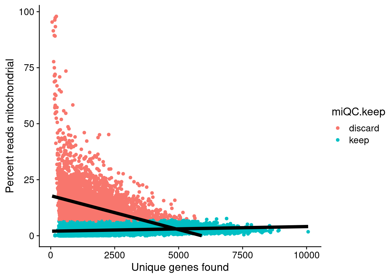
| Version | Author | Date |
|---|---|---|
| b47d7b0 | Florian Wuennemann | 2022-03-24 |
Apply filters
After calculating mitochondrial read thresholds, let’s now actual filter out low quality cells based on some arbitrary manual thresholds for minimum number of genes and based on miQC classification.
## Filter based on miQC suggestion
seurat_object_filt <- subset(seurat_object, miQC.keep == "keep")

## Filter out cells with low number of genes
seurat_object_filt <- subset(seurat_object, subset = nFeature_RNA > 200 & nFeature_RNA < 6000)
Process and integrate data
Now that we have clean data, we run a standard Seurat clustering analysis, followed by integration of the data using the Harmony method.
Seurat and Harmony
## Since these analyses take some time, only run them if the analysis has not been performed prio
if(!file.exists(seurat_object_file)){
  seurat_object_filt <- NormalizeData(seurat_object_filt) %>% FindVariableFeatures() %>%
    ScaleData() %>% RunPCA(verbose = FALSE)

  ElbowPlot(seurat_object_filt, ndims = 50)

  seurat_object_filt <- RunHarmony(seurat_object_filt, group.by.vars = "group")
  seurat_object_filt <- RunUMAP(seurat_object_filt, reduction = "harmony", dims = 1:20)
  seurat_object_filt <- FindNeighbors(seurat_object_filt, reduction = "harmony", dims = 1:20) %>% FindClusters()
}else{
  seurat_object_filt <- readRDS(seurat_object_file)
}
Plot cell embeddings
After processing the data, let’s visualize the cell embeddings returned by Harmony. Please keep in mind, that cluster numbers here are arbitrary from the nearest neighbour algorithm and do not correspond to cluster numbers from other, previous clusterings.
DimPlot(seurat_object_filt, group.by = c("seurat_clusters"), label = TRUE)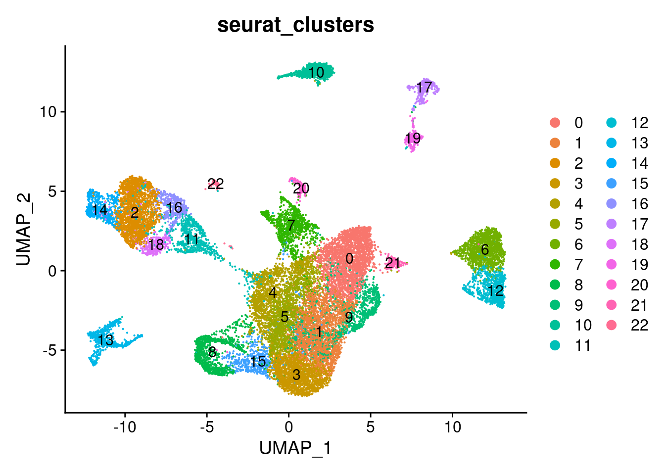
DimPlot(seurat_object_filt, group.by = "group")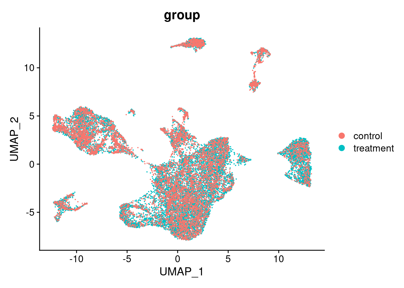
| Version | Author | Date |
|---|---|---|
| 29960c2 | Florian Wuennemann | 2022-03-24 |
Save Seurat object
Finally, let’s save our final, processed Seurat object to load it in later analysis.
## Only save seurat object if it has not been computed before
if(!file.exists(seurat_object_file)){
  saveRDS(seurat_object_filt,
        file = seurat_object_file)
}
sessionInfo()R version 4.1.3 (2022-03-10)
Platform: x86_64-pc-linux-gnu (64-bit)
Running under: Ubuntu 20.04.4 LTS
Matrix products: default
BLAS: /usr/lib/x86_64-linux-gnu/blas/libblas.so.3.9.0
LAPACK: /usr/lib/x86_64-linux-gnu/lapack/liblapack.so.3.9.0
locale:
[1] LC_CTYPE=en_US.UTF-8 LC_NUMERIC=C
[3] LC_TIME=de_DE.UTF-8 LC_COLLATE=en_US.UTF-8
[5] LC_MONETARY=de_DE.UTF-8 LC_MESSAGES=en_US.UTF-8
[7] LC_PAPER=de_DE.UTF-8 LC_NAME=C
[9] LC_ADDRESS=C LC_TELEPHONE=C
[11] LC_MEASUREMENT=de_DE.UTF-8 LC_IDENTIFICATION=C
attached base packages:
[1] splines stats4 stats graphics grDevices utils datasets
[8] methods base
other attached packages:
[1] biomaRt_2.51.3 flexmix_2.3-17
[3] lattice_0.20-45 scater_1.22.0
[5] ggplot2_3.3.5 scuttle_1.4.0
[7] scRNAseq_2.8.0 SingleCellExperiment_1.16.0
[9] SummarizedExperiment_1.24.0 Biobase_2.54.0
[11] GenomicRanges_1.46.1 GenomeInfoDb_1.30.1
[13] IRanges_2.28.0 S4Vectors_0.32.4
[15] BiocGenerics_0.40.0 MatrixGenerics_1.7.0
[17] matrixStats_0.61.0 harmony_0.1.0
[19] Rcpp_1.0.8.3 SeuratWrappers_0.3.0
[21] miQC_1.2.0 hdf5r_1.3.5
[23] SeuratObject_4.0.4 Seurat_4.1.0
[25] workflowr_1.7.0
loaded via a namespace (and not attached):
[1] rappdirs_0.3.3 rtracklayer_1.54.0
[3] scattermore_0.8 R.methodsS3_1.8.1
[5] tidyr_1.2.0 bit64_4.0.5
[7] knitr_1.38 irlba_2.3.5
[9] DelayedArray_0.20.0 R.utils_2.11.0
[11] data.table_1.14.2 rpart_4.1.16
[13] KEGGREST_1.34.0 RCurl_1.98-1.6
[15] AnnotationFilter_1.18.0 generics_0.1.2
[17] GenomicFeatures_1.46.5 ScaledMatrix_1.2.0
[19] callr_3.7.0 cowplot_1.1.1
[21] RSQLite_2.2.12 RANN_2.6.1
[23] future_1.24.0 bit_4.0.4
[25] spatstat.data_2.1-4 xml2_1.3.3
[27] httpuv_1.6.5 assertthat_0.2.1
[29] viridis_0.6.2 xfun_0.30
[31] hms_1.1.1 jquerylib_0.1.4
[33] evaluate_0.15 promises_1.2.0.1
[35] fansi_1.0.3 restfulr_0.0.13
[37] progress_1.2.2 dbplyr_2.1.1
[39] igraph_1.3.0 DBI_1.1.2
[41] htmlwidgets_1.5.4 spatstat.geom_2.4-0
[43] purrr_0.3.4 ellipsis_0.3.2
[45] dplyr_1.0.8 deldir_1.0-6
[47] sparseMatrixStats_1.7.0 vctrs_0.4.1
[49] remotes_2.4.2 ensembldb_2.18.4
[51] ROCR_1.0-11 abind_1.4-5
[53] cachem_1.0.6 withr_2.5.0
[55] sctransform_0.3.3 GenomicAlignments_1.30.0
[57] prettyunits_1.1.1 goftest_1.2-3
[59] cluster_2.1.3 ExperimentHub_2.2.1
[61] lazyeval_0.2.2 crayon_1.5.1
[63] labeling_0.4.2 pkgconfig_2.0.3
[65] vipor_0.4.5 nlme_3.1-157
[67] ProtGenerics_1.26.0 nnet_7.3-17
[69] rlang_1.0.2 globals_0.14.0
[71] lifecycle_1.0.1 miniUI_0.1.1.1
[73] filelock_1.0.2 BiocFileCache_2.2.1
[75] rsvd_1.0.5 AnnotationHub_3.2.2
[77] rprojroot_2.0.3 polyclip_1.10-0
[79] lmtest_0.9-40 Matrix_1.4-1
[81] zoo_1.8-9 beeswarm_0.4.0
[83] whisker_0.4 ggridges_0.5.3
[85] processx_3.5.3 png_0.1-7
[87] viridisLite_0.4.0 rjson_0.2.21
[89] bitops_1.0-7 getPass_0.2-2
[91] R.oo_1.24.0 KernSmooth_2.23-20
[93] Biostrings_2.62.0 blob_1.2.3
[95] DelayedMatrixStats_1.16.0 stringr_1.4.0
[97] parallelly_1.31.0 spatstat.random_2.2-0
[99] beachmat_2.10.0 scales_1.2.0
[101] memoise_2.0.1 magrittr_2.0.3
[103] plyr_1.8.7 ica_1.0-2
[105] zlibbioc_1.40.0 compiler_4.1.3
[107] BiocIO_1.4.0 RColorBrewer_1.1-3
[109] fitdistrplus_1.1-8 Rsamtools_2.10.0
[111] cli_3.2.0 XVector_0.34.0
[113] listenv_0.8.0 patchwork_1.1.1
[115] pbapply_1.5-0 ps_1.6.0
[117] MASS_7.3-56 mgcv_1.8-40
[119] tidyselect_1.1.2 stringi_1.7.6
[121] highr_0.9 yaml_2.3.5
[123] BiocSingular_1.10.0 ggrepel_0.9.1
[125] grid_4.1.3 sass_0.4.1
[127] tools_4.1.3 future.apply_1.8.1
[129] parallel_4.1.3 rstudioapi_0.13
[131] git2r_0.30.1 gridExtra_2.3
[133] farver_2.1.0 Rtsne_0.15
[135] digest_0.6.29 BiocManager_1.30.16
[137] shiny_1.7.1 BiocVersion_3.14.0
[139] later_1.3.0 RcppAnnoy_0.0.19
[141] httr_1.4.2 AnnotationDbi_1.56.2
[143] colorspace_2.0-3 XML_3.99-0.9
[145] fs_1.5.2 tensor_1.5
[147] reticulate_1.24 uwot_0.1.11
[149] spatstat.utils_2.3-0 plotly_4.10.0
[151] xtable_1.8-4 jsonlite_1.8.0
[153] modeltools_0.2-23 R6_2.5.1
[155] pillar_1.7.0 htmltools_0.5.2
[157] mime_0.12 glue_1.6.2
[159] fastmap_1.1.0 BiocParallel_1.28.3
[161] BiocNeighbors_1.12.0 interactiveDisplayBase_1.32.0
[163] codetools_0.2-18 utf8_1.2.2
[165] bslib_0.3.1 spatstat.sparse_2.1-0
[167] tibble_3.1.6 curl_4.3.2
[169] ggbeeswarm_0.6.0 leiden_0.3.9
[171] survival_3.2-13 rmarkdown_2.13
[173] munsell_0.5.0 GenomeInfoDbData_1.2.7
[175] reshape2_1.4.4 gtable_0.3.0
[177] spatstat.core_2.4-2