- Aim
- Load data
- Perform DE using manual pseudobulking of counts and DESeq2
- Run DESeq2 per cell type
- Check the most significant DE genes
- Plot Volcano plot of pseudobulk results
- Check relationship between baseMean expression and log2FC
- Compare results to results from FindMarker wilcoxon test
- Save merged table for future use
Differential expression analysis using pseudobulks
Florian Wuenenmann
3/10/2022
Last updated: 2022-04-19
Checks: 7 0
Knit directory: Abatacept_scrnaseq_mi/
This reproducible R Markdown analysis was created with workflowr (version 1.7.0). The Checks tab describes the reproducibility checks that were applied when the results were created. The Past versions tab lists the development history.
Great! Since the R Markdown file has been committed to the Git repository, you know the exact version of the code that produced these results.
Great job! The global environment was empty. Objects defined in the global environment can affect the analysis in your R Markdown file in unknown ways. For reproduciblity it’s best to always run the code in an empty environment.
The command set.seed(20220318) was run prior to running the code in the R Markdown file. Setting a seed ensures that any results that rely on randomness, e.g. subsampling or permutations, are reproducible.
Great job! Recording the operating system, R version, and package versions is critical for reproducibility.
Nice! There were no cached chunks for this analysis, so you can be confident that you successfully produced the results during this run.
Great job! Using relative paths to the files within your workflowr project makes it easier to run your code on other machines.
Great! You are using Git for version control. Tracking code development and connecting the code version to the results is critical for reproducibility.
The results in this page were generated with repository version 6fc473c. See the Past versions tab to see a history of the changes made to the R Markdown and HTML files.
Note that you need to be careful to ensure that all relevant files for the analysis have been committed to Git prior to generating the results (you can use wflow_publish or wflow_git_commit). workflowr only checks the R Markdown file, but you know if there are other scripts or data files that it depends on. Below is the status of the Git repository when the results were generated:
Ignored files:
    Ignored:    .Rhistory
    Ignored:    .Rproj.user/

Untracked files:
    Untracked:  code/utils.R
    Untracked:  code/utils_nichenet.R
    Untracked:  data/Table_1_Common Transcriptomic Effects of Abatacept and Other DMARDs on Rheumatoid Arthritis Synovial Tissue.xlsx
    Untracked:  omnipathr-log/

Unstaged changes:
    Deleted:    analysis/7_Conclusions.Rmd
    Deleted:    analysis/7_summary.Rmd
Note that any generated files, e.g. HTML, png, CSS, etc., are not included in this status report because it is ok for generated content to have uncommitted changes.
These are the previous versions of the repository in which changes were made to the R Markdown (analysis/3_differential_pseudobulk_analysis.Rmd) and HTML (docs/3_differential_pseudobulk_analysis.html) files. If you’ve configured a remote Git repository (see ?wflow_git_remote), click on the hyperlinks in the table below to view the files as they were in that past version.
| File | Version | Author | Date | Message |
|---|---|---|---|---|
| html | a71b19c | Florian Wuennemann | 2022-04-19 | Build site. |
| Rmd | 86ff3e7 | Florian Wuennemann | 2022-04-19 | Main Update to code and adding NichenetR |
| html | 6e3bb2f | Florian Wuennemann | 2022-03-25 | Build site. |
| html | 8193696 | Florian Wuennemann | 2022-03-25 | Build site. |
| Rmd | ea7721d | Florian Wuennemann | 2022-03-25 | wflow_publish("analysis/3_differential_pseudobulk_analysis.Rmd") |
| html | d75734d | Florian Wuennemann | 2022-03-25 | Build site. |
| Rmd | 25b6b09 | Florian Wuennemann | 2022-03-25 | wflow_publish("analysis/3_differential_pseudobulk_analysis.Rmd") |
| html | b47d7b0 | Florian Wuennemann | 2022-03-24 | Build site. |
| Rmd | 8591656 | Florian Wuennemann | 2022-03-24 | wflow_publish(c("analysis/1_process_and_integrate_Seurat_Harmony.Rmd", |
| html | 46f2db7 | Florian Wuennemann | 2022-03-23 | First commit. |
Aim
Estimating differential expression while incorporating replicate information in single-cell analyses is an ongoing, unsolved topic. Recent discussions have highlighted that the best approaches are pseudobulk approaches using established RNA-seq packages such as DESeq2 and mixed models incorporating the replicate information in the models.
Recent preprints and publications discussing this in detail can be found here:
Load data
First,we load our Seurat object processed with Harmony again.
seurat_object_filt <- readRDS(here("../data/2_annotated.seurat_object.rds"))Perform DE using manual pseudobulking of counts and DESeq2
For each cell type, we will create pseudobulk expression samples by replicate (using the sum of counts) and then use DEseq2 to perform differential expression between the control and treatment samples. To create Pseudobulks, we will sum up all UMI counts per replicate and perform normalizaion with DESeq2.
Run DESeq2 per cell type
## Only run DE analysis if it hasnt been computed yet
pseudobulk_de_file <- here("../results/3_DE_genes.pseudobulk_results.tsv")

## Only run analysis if it hasn't been calculated yet
if(file.exists(pseudobulk_de_file)){
  all_de <- fread(pseudobulk_de_file)
}else{
  cell_types <- unique(seurat_object_filt@meta.data$cell_type)

  all_de <- data.frame()
  counter <- 0
  for(this_type in cell_types){
    counter <- counter + 1
    print(paste(counter,":",this_type,sep =""))

    ## Subset seurat object for cell type to be analyzed and create pseudobulks using mean expression per replicate
    seurat_sub <- subset(seurat_object_filt,cell_type == this_type)
    seurat_sub_avg <- AggregateExpression(object = seurat_sub,
                                        assays = "RNA",
                                        group.by = "orig.ident",
                                        slot = "counts")

    metadata <- seurat_sub@meta.data %>%
      dplyr::select(orig.ident,group) %>%
      unique()
    rownames(metadata) <- metadata$orig.ident

    metadata <- metadata %>% dplyr::select(-orig.ident)%>% mutate("group" = as.factor(group))
    metadata$seq_lane <- c("R1","R2","R1","R2")

    ## Run DE using DESeq2
    dds <- DESeqDataSetFromMatrix(seurat_sub_avg$RNA,
                                colData = metadata,
                                design = ~ group)

    rld <- rlog(dds, blind=FALSE)

    # Run DESeq2 differential expression analysis
    dds <- DESeq(dds)

               # Plot dispersion estimates

    contrast <- c("group", "treatment", "control")

    # resultsNames(dds)
    res <- results(dds,
                   contrast = contrast,
                   alpha = 0.05)

    res <- lfcShrink(dds,
                     coef =  "group_treatment_vs_control",
                     res=res)

    # Turn the results object into a tibble for use with tidyverse functions
    res_tbl <- res %>%
            data.frame() %>%
            rownames_to_column(var="gene") %>%
            as_tibble() %>%
            arrange(padj)

    ## Add cell type as column
    res_tbl$cell_type <- this_type

    all_de <- rbind(all_de,res_tbl)
  }

  all_de <- all_de %>%
    arrange(padj)

  write.table(all_de,
              file = pseudobulk_de_file,
              sep = "\t",
              col.names = TRUE,
              quote = FALSE,
              row.names = FALSE)
}
Check the most significant DE genes
Now that we have calculated the differentially expressed genes, based on pseudobulks of cell types, let’s see how many we identified and which ones for each cell type. Please note, that due to the fact that we only have 2 replicates per group, the number of DE genes estimated will be very conservative and thus much lower compared to a wilcoxon test performed on individual cells.
## Get all significant genes
sig_genes <- all_de %>%
  subset(padj < 0.05) %>%
  arrange(log2FoldChange)

dim(sig_genes)
[1] 269 7sig_genes_per_ct <- sig_genes %>%
group_by(cell_type) %>%
tally() %>%
arrange(desc(n))
sig_genes_per_ct# A tibble: 14 × 2
cell_type n
<chr> <int>
1 Fib_act 156
2 Mac_3 23
3 Mac_IFNIC 21
4 Fib_3 15
5 Fib_cyc 15
6 Mac_TR 14
7 Mac_1 10
8 Mac_2 5
9 EC 3
10 NK 3
11 B 1
12 DC_1 1
13 DC_2 1
14 Mono_1 1Plot Volcano plot of pseudobulk results
Let’s plot a volcano plot per cell-type. Remember that the adjusted p-values will be very conservative. We are only plotting genes with adjusted p-values < 0.05 since otherwise the interactive plot will be very slow.
library(plotly)
Attaching package: 'plotly'The following object is masked from 'package:ggplot2':
last_plotThe following object is masked from 'package:IRanges':
sliceThe following object is masked from 'package:S4Vectors':
renameThe following object is masked from 'package:stats':
filterThe following object is masked from 'package:graphics':
layoutall_de_plot <- all_de %>%
group_by(cell_type) %>%
mutate("de_cell_rank" = order(-log10(padj), decreasing = TRUE))
volcano_pot <- ggplot(all_de_plot,aes(log2FoldChange,-log10(padj),text = gene)) +
#geom_point(data = subset(all_de_plot, padj > 0.05)) +
geom_point(data = subset(all_de_plot, padj <= 0.05)) +
facet_wrap(~ cell_type) +
theme_bw() +
geom_hline(yintercept = -log10(0.05), linetype = 2) +
geom_vline(xintercept = 0)
ggplotly(volcano_pot)Warning: `gather_()` was deprecated in tidyr 1.2.0.
Please use `gather()` instead.
This warning is displayed once every 8 hours.
Call `lifecycle::last_lifecycle_warnings()` to see where this warning was generated.Check relationship between baseMean expression and log2FC
Let’s quickly visualize the relationship between the base expression of a gene and the log2 fold-change determined by DESeq2. In general, we expect the the log2FC to be stronger when the base-expression is lower, as smaller differences between control and treatment samples will be relatively stronger.
ggplot() +
  geom_point(data = subset(all_de,padj > 0.05),
             aes(baseMean,log2FoldChange),color = "darkgrey") +
  geom_point(data = subset(all_de,padj <= 0.05),
             aes(baseMean,log2FoldChange),color = "red") +
  facet_wrap(~ cell_type)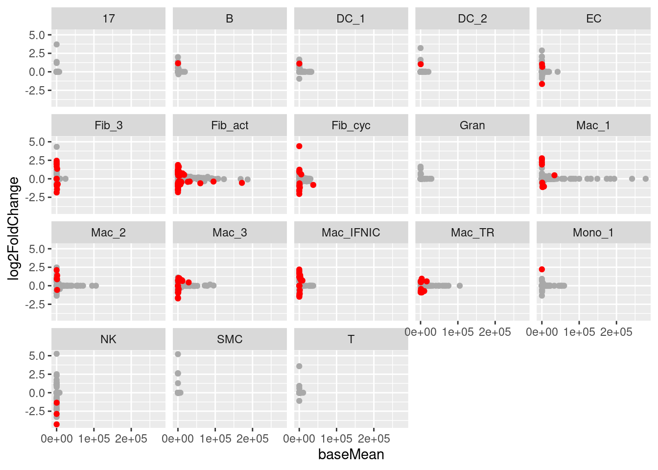
Compare results to results from FindMarker wilcoxon test
Finally, let’s actually compare the initial DE results using the wilcoxon rank sum test with the pseudobulk DE-seq results. We expect adjusted p-values from the wilcoxon test to be highly inflated.
## Load all de results and merge into one big table for comparison
de_file_dir <- list.files(here("../DE_lists"))
orig_de <- data.frame()

for(filename in de_file_dir){
  print(filename)
  file_dat <- fread(paste(here("../DE_lists"),filename,sep="/"))
  file_dat$file <- filename
  orig_de <- rbind(orig_de,file_dat)
  }
[1] "DEGS_17.csv"
[1] "DEGS_B.csv"
[1] "DEGS_DC_1.csv"
[1] "DEGS_DC_2.csv"
[1] "DEGS_EC.csv"
[1] "DEGS_Fib_3.csv"
[1] "DEGS_Fib_act.csv"
[1] "DEGS_Fib_cyc.csv"
[1] "DEGS_Gran.csv"
[1] "DEGS_Mac_2.csv"
[1] "DEGS_Mac_3.csv"
[1] "DEGS_Mac_IFNIC.csv"
[1] "DEGS_Mac_TR.csv"
[1] "DEGS_Mono_1.csv"
[1] "DEGS_NK.csv"
[1] "DEGS_SMC.csv"
[1] "DEGS_T.csv"colnames(orig_de) <- gsub("V1","gene",colnames(orig_de))
orig_de_mod <- orig_de %>%
mutate("cell_type" = gsub("DEGS_","",file)) %>%
mutate("cell_type" = gsub(".csv","",cell_type)) %>%
arrange(p_val_adj)
orig_de_mod_sig <- orig_de_mod %>%
subset(p_val_adj < 0.05) %>%
arrange(desc(avg_log2FC))merged_de <- full_join(all_de,orig_de_mod,by = c("cell_type","gene"),
suffix = c(".pseudobulk",".wilcox"))
merged_de <- merged_de %>%
mutate("logFC_dif" = log2FoldChange - avg_log2FC) %>%
arrange(logFC_dif)## Plot -log10 p-values from different DE approaches
ggplot(merged_de,aes(-log10(padj),-log10(p_val_adj), color = logFC_dif)) +
geom_point() +
geom_abline() +
theme_bw() +
scale_color_viridis_c() +
labs(x = "-log10(p-value) DESeq2 pseudobulk",#
y = "-log10(p-value) Wilcoxon test on single-cells")Warning: Removed 349759 rows containing missing values (geom_point).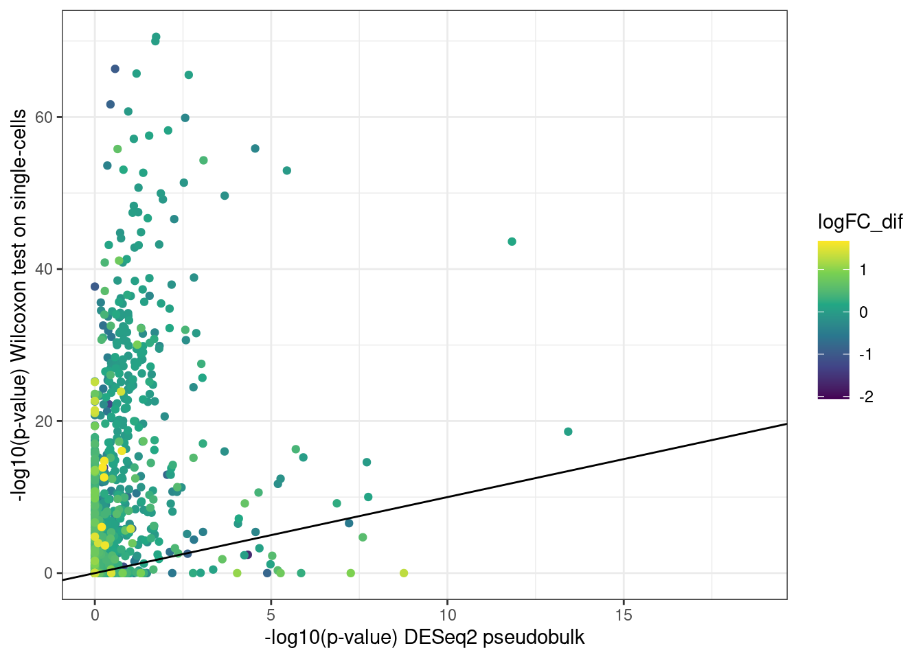
| Version | Author | Date |
|---|---|---|
| a71b19c | Florian Wuennemann | 2022-04-19 |
ggplot(merged_de,aes(log2FoldChange,avg_log2FC, color = logFC_dif)) +
  geom_point() +
  geom_abline() +
  theme_bw() +
  scale_color_viridis_c() +
  labs(x = "log2FoldChange DESeq2 pseudobulk",#
       y = "log2FoldChange Wilcoxon test on single-cells")
Warning: Removed 349729 rows containing missing values (geom_point).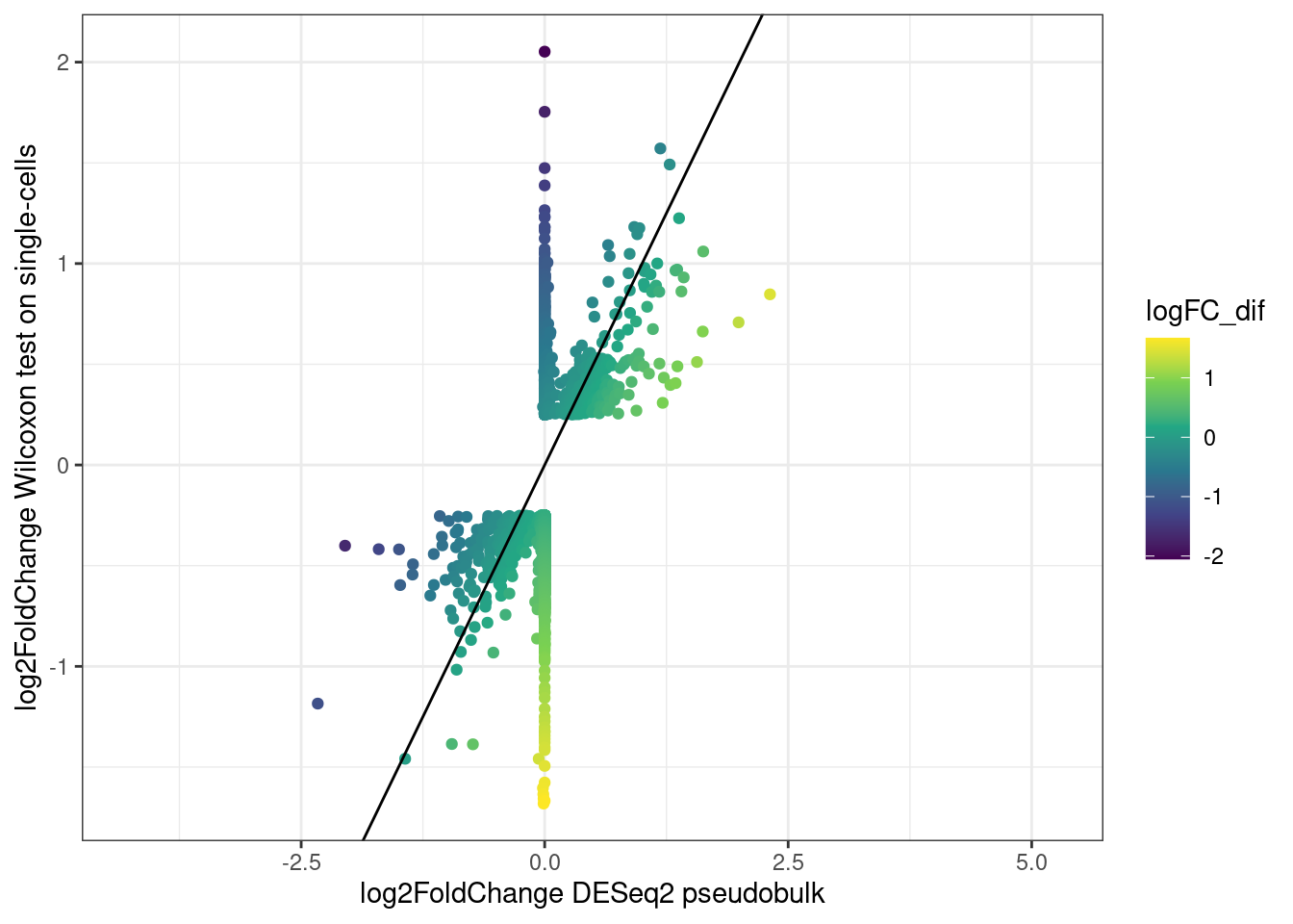
| Version | Author | Date |
|---|---|---|
| a71b19c | Florian Wuennemann | 2022-04-19 |
As we can see, indeed the p-values from the wilcoxon test are very inflated compared to the more conservative pseudobulk results.
Let’s look at the difference in number of differentially expressed genes using both approaches.
## Compare number of DE genes between both approaches
pseudobulk_num <- all_de %>%
  subset(padj < 0.05) %>%
  group_by(cell_type) %>%
  tally()

wilcoxon_num <- orig_de_mod %>%
  subset(p_val_adj < 0.05) %>%
  group_by(cell_type) %>%
  tally()

merge_counts <- full_join(pseudobulk_num,wilcoxon_num,by = "cell_type")
merge_counts[is.na(merge_counts)] <- 0

colnames(merge_counts) <- c("cell_type","n_genes_pseudobulk","n_genes_wilcoxon")
merge_counts <- merge_counts %>%
  mutate("difference" = n_genes_wilcoxon - n_genes_pseudobulk) %>%
  arrange(desc(difference))

reactable(merge_counts)Save merged table for future use
write.table(merged_de,
            file = here("../results/3_DE_genes.merged_wilcox_pseudobulk.tsv"),
            sep = "\t",
            col.names = TRUE,
            quote = FALSE,
            row.names = FALSE)
sessionInfo()R version 4.1.3 (2022-03-10)
Platform: x86_64-pc-linux-gnu (64-bit)
Running under: Ubuntu 20.04.4 LTS
Matrix products: default
BLAS: /usr/lib/x86_64-linux-gnu/blas/libblas.so.3.9.0
LAPACK: /usr/lib/x86_64-linux-gnu/lapack/liblapack.so.3.9.0
locale:
[1] LC_CTYPE=en_US.UTF-8 LC_NUMERIC=C
[3] LC_TIME=de_DE.UTF-8 LC_COLLATE=en_US.UTF-8
[5] LC_MONETARY=de_DE.UTF-8 LC_MESSAGES=en_US.UTF-8
[7] LC_PAPER=de_DE.UTF-8 LC_NAME=C
[9] LC_ADDRESS=C LC_TELEPHONE=C
[11] LC_MEASUREMENT=de_DE.UTF-8 LC_IDENTIFICATION=C
attached base packages:
[1] stats4 stats graphics grDevices utils datasets methods
[8] base
other attached packages:
[1] plotly_4.10.0 ggridges_0.5.3
[3] here_1.0.1 reactable_0.2.3
[5] patchwork_1.1.1 aggregateBioVar_1.4.0
[7] data.table_1.14.2 forcats_0.5.1
[9] stringr_1.4.0 dplyr_1.0.8
[11] purrr_0.3.4 readr_2.1.2
[13] tidyr_1.2.0 tibble_3.1.6
[15] ggplot2_3.3.5 tidyverse_1.3.1
[17] DESeq2_1.34.0 SummarizedExperiment_1.24.0
[19] Biobase_2.54.0 MatrixGenerics_1.7.0
[21] matrixStats_0.61.0 GenomicRanges_1.46.1
[23] GenomeInfoDb_1.30.1 IRanges_2.28.0
[25] S4Vectors_0.32.4 BiocGenerics_0.40.0
[27] SeuratObject_4.0.4 Seurat_4.1.0
[29] workflowr_1.7.0
loaded via a namespace (and not attached):
[1] utf8_1.2.2 R.utils_2.11.0
[3] reticulate_1.24 tidyselect_1.1.2
[5] RSQLite_2.2.12 AnnotationDbi_1.56.2
[7] htmlwidgets_1.5.4 grid_4.1.3
[9] BiocParallel_1.28.3 Rtsne_0.15
[11] munsell_0.5.0 codetools_0.2-18
[13] ica_1.0-2 future_1.24.0
[15] miniUI_0.1.1.1 withr_2.5.0
[17] spatstat.random_2.2-0 colorspace_2.0-3
[19] highr_0.9 knitr_1.38
[21] rstudioapi_0.13 SingleCellExperiment_1.16.0
[23] ROCR_1.0-11 tensor_1.5
[25] listenv_0.8.0 labeling_0.4.2
[27] git2r_0.30.1 GenomeInfoDbData_1.2.7
[29] polyclip_1.10-0 farver_2.1.0
[31] bit64_4.0.5 rprojroot_2.0.3
[33] parallelly_1.31.0 vctrs_0.4.1
[35] generics_0.1.2 xfun_0.30
[37] R6_2.5.1 rsvd_1.0.5
[39] locfit_1.5-9.5 flexmix_2.3-17
[41] bitops_1.0-7 spatstat.utils_2.3-0
[43] cachem_1.0.6 DelayedArray_0.20.0
[45] assertthat_0.2.1 promises_1.2.0.1
[47] scales_1.2.0 nnet_7.3-17
[49] gtable_0.3.0 globals_0.14.0
[51] processx_3.5.3 goftest_1.2-3
[53] rlang_1.0.2 genefilter_1.76.0
[55] splines_4.1.3 lazyeval_0.2.2
[57] spatstat.geom_2.4-0 broom_0.8.0
[59] BiocManager_1.30.16 yaml_2.3.5
[61] reshape2_1.4.4 abind_1.4-5
[63] modelr_0.1.8 crosstalk_1.2.0
[65] backports_1.4.1 httpuv_1.6.5
[67] tools_4.1.3 ellipsis_0.3.2
[69] spatstat.core_2.4-2 jquerylib_0.1.4
[71] RColorBrewer_1.1-3 Rcpp_1.0.8.3
[73] plyr_1.8.7 zlibbioc_1.40.0
[75] RCurl_1.98-1.6 ps_1.6.0
[77] rpart_4.1.16 deldir_1.0-6
[79] pbapply_1.5-0 cowplot_1.1.1
[81] zoo_1.8-9 reactR_0.4.4
[83] haven_2.4.3 ggrepel_0.9.1
[85] cluster_2.1.3 fs_1.5.2
[87] magrittr_2.0.3 scattermore_0.8
[89] reprex_2.0.1 lmtest_0.9-40
[91] RANN_2.6.1 whisker_0.4
[93] fitdistrplus_1.1-8 hms_1.1.1
[95] mime_0.12 evaluate_0.15
[97] xtable_1.8-4 XML_3.99-0.9
[99] readxl_1.4.0 gridExtra_2.3
[101] compiler_4.1.3 KernSmooth_2.23-20
[103] crayon_1.5.1 R.oo_1.24.0
[105] htmltools_0.5.2 mgcv_1.8-40
[107] later_1.3.0 tzdb_0.3.0
[109] geneplotter_1.72.0 lubridate_1.8.0
[111] DBI_1.1.2 dbplyr_2.1.1
[113] MASS_7.3-56 Matrix_1.4-1
[115] cli_3.2.0 R.methodsS3_1.8.1
[117] parallel_4.1.3 igraph_1.3.0
[119] pkgconfig_2.0.3 getPass_0.2-2
[121] spatstat.sparse_2.1-0 xml2_1.3.3
[123] annotate_1.72.0 bslib_0.3.1
[125] XVector_0.34.0 rvest_1.0.2
[127] callr_3.7.0 digest_0.6.29
[129] sctransform_0.3.3 RcppAnnoy_0.0.19
[131] spatstat.data_2.1-4 Biostrings_2.62.0
[133] rmarkdown_2.13 cellranger_1.1.0
[135] leiden_0.3.9 uwot_0.1.11
[137] modeltools_0.2-23 shiny_1.7.1
[139] lifecycle_1.0.1 nlme_3.1-157
[141] jsonlite_1.8.0 SeuratWrappers_0.3.0
[143] viridisLite_0.4.0 fansi_1.0.3
[145] pillar_1.7.0 lattice_0.20-45
[147] KEGGREST_1.34.0 fastmap_1.1.0
[149] httr_1.4.2 survival_3.2-13
[151] remotes_2.4.2 glue_1.6.2
[153] png_0.1-7 bit_4.0.4
[155] stringi_1.7.6 sass_0.4.1
[157] blob_1.2.3 memoise_2.0.1
[159] irlba_2.3.5 future.apply_1.8.1