5 Augur cell prioritization
Florian Wuenenmann
3/15/2022
Last updated: 2022-04-19
Checks: 7 0
Knit directory: Abatacept_scrnaseq_mi/
This reproducible R Markdown analysis was created with workflowr (version 1.7.0). The Checks tab describes the reproducibility checks that were applied when the results were created. The Past versions tab lists the development history.
Great! Since the R Markdown file has been committed to the Git repository, you know the exact version of the code that produced these results.
Great job! The global environment was empty. Objects defined in the global environment can affect the analysis in your R Markdown file in unknown ways. For reproduciblity it’s best to always run the code in an empty environment.
The command set.seed(20220318) was run prior to running the code in the R Markdown file. Setting a seed ensures that any results that rely on randomness, e.g. subsampling or permutations, are reproducible.
Great job! Recording the operating system, R version, and package versions is critical for reproducibility.
Nice! There were no cached chunks for this analysis, so you can be confident that you successfully produced the results during this run.
Great job! Using relative paths to the files within your workflowr project makes it easier to run your code on other machines.
Great! You are using Git for version control. Tracking code development and connecting the code version to the results is critical for reproducibility.
The results in this page were generated with repository version 6fc473c. See the Past versions tab to see a history of the changes made to the R Markdown and HTML files.
Note that you need to be careful to ensure that all relevant files for the analysis have been committed to Git prior to generating the results (you can use wflow_publish or wflow_git_commit). workflowr only checks the R Markdown file, but you know if there are other scripts or data files that it depends on. Below is the status of the Git repository when the results were generated:
Ignored files:
    Ignored:    .Rhistory
    Ignored:    .Rproj.user/

Untracked files:
    Untracked:  code/utils.R
    Untracked:  code/utils_nichenet.R
    Untracked:  data/Table_1_Common Transcriptomic Effects of Abatacept and Other DMARDs on Rheumatoid Arthritis Synovial Tissue.xlsx
    Untracked:  omnipathr-log/

Unstaged changes:
    Deleted:    analysis/7_Conclusions.Rmd
    Deleted:    analysis/7_summary.Rmd
Note that any generated files, e.g. HTML, png, CSS, etc., are not included in this status report because it is ok for generated content to have uncommitted changes.
These are the previous versions of the repository in which changes were made to the R Markdown (analysis/4_run_augur_prioritization.Rmd) and HTML (docs/4_run_augur_prioritization.html) files. If you’ve configured a remote Git repository (see ?wflow_git_remote), click on the hyperlinks in the table below to view the files as they were in that past version.
| File | Version | Author | Date | Message |
|---|---|---|---|---|
| html | a71b19c | Florian Wuennemann | 2022-04-19 | Build site. |
| Rmd | 86ff3e7 | Florian Wuennemann | 2022-04-19 | Main Update to code and adding NichenetR |
| html | 6e3bb2f | Florian Wuennemann | 2022-03-25 | Build site. |
| Rmd | 3a8a835 | Florian Wuennemann | 2022-03-25 | wflow_publish("analysis/*") |
| html | b47d7b0 | Florian Wuennemann | 2022-03-24 | Build site. |
| Rmd | 8591656 | Florian Wuennemann | 2022-03-24 | wflow_publish(c("analysis/1_process_and_integrate_Seurat_Harmony.Rmd", |
| html | 46f2db7 | Florian Wuennemann | 2022-03-23 | First commit. |
Run Augur on processed single-cell data
Aim
In this analysis, we will use AUGUR to prioritize cell-types, based on how much they are affected by the treatment with Abatacept. The approach of AUGUR uses random-forest classifiers to try to predict the treatment group of each cell per cell-type and calculates an area-under-the-curve (AUC) to describe how well it performs. We can interpret this AUC as how much the treatment and control groups can be distinguished based on their differences (i.e. how much does treatment affect a cell-type).
Run AUGUR on Seurat object
First, as usual, let’s read the Seurat object.
seurat_object_filt <- readRDS(here("../data/2_annotated.seurat_object.rds"))Then, we run AUGUR or read the augur results if they have already be calculated.
augur_object_name <- here("../results/4_augur.harmony_seurat_object.rds")
if(file.exists(augur_object_name)){ ## IF results have been computed, read the object
  augur <- readRDS(augur_object_name)
}else{
  augur = calculate_auc(seurat_object_filt, seurat_object_filt@meta.data,
                      cell_type_col = "cell_type", label_col = "group")
  saveRDS(augur,
        file = augur_object_name)
}
Visualize augur results to find most affected cell types
Let’s look at the main result of AUGUR, the AUCs for classifying cells into treatment groups for the different cell types. The highest ranked cell type here is the one that is predicted to be the most affected by the treatment based on AUGURs method.
## Get color palette for cell types that fits Seurats color plotting
## From: https://github.com/satijalab/seurat/issues/257
# Create vector with levels of object@ident
identities <- levels(seurat_object_filt@active.ident)
# Create vector of default ggplot2 colors
my_color_palette <- hue_pal()(length(identities))


plot_lollipop(augur) +
  geom_point(aes(color = cell_type), size = 3) +
  theme(legend.position = "none") +
  scale_color_manual(values = my_color_palette)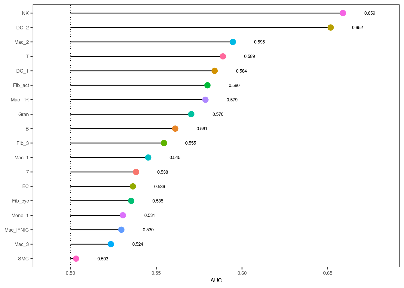
| Version | Author | Date |
|---|---|---|
| 6e3bb2f | Florian Wuennemann | 2022-03-25 |
plot_umap(augur,sc = seurat_object_filt)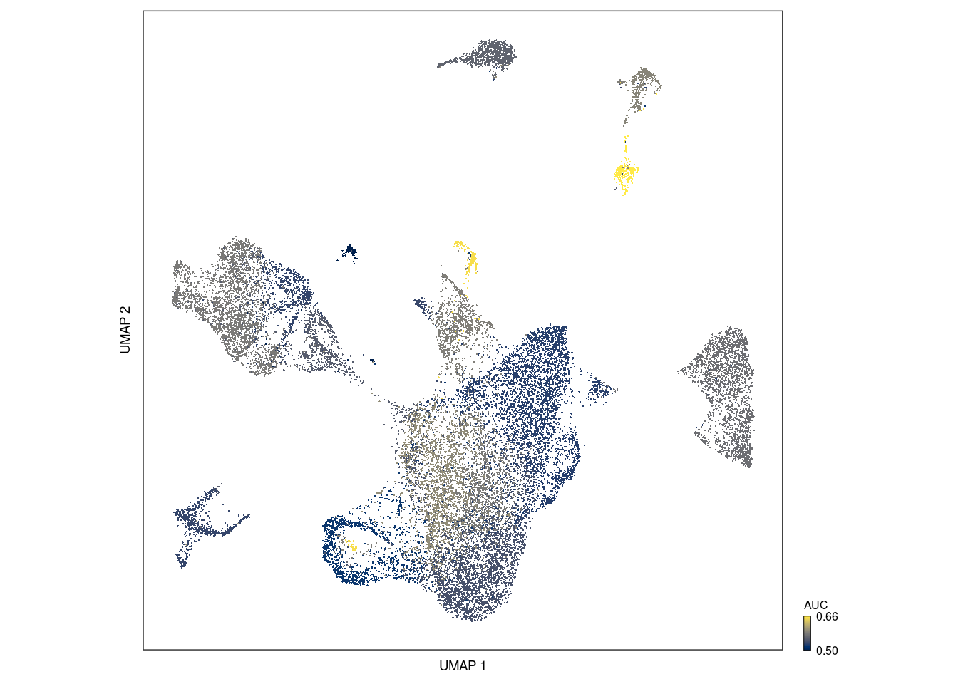
Compare AUGUR AUC with number of DE genes based on p-values
Finally, let’s see whether the AUC calculated by AUGUR correlates with the number of statistically significant differentially expressed genes.
de_genes <- fread(here("../results/3_DE_genes.pseudobulk_results.tsv"))

de_genes_per_ct <- de_genes %>%
  subset(padj <= 0.05) %>%
  group_by(cell_type) %>%
  tally() %>%
  arrange(desc(n))
auc_ct <- augur$AUC
merged_augur_stats <- full_join(auc_ct,de_genes_per_ct,by = "cell_type")ggplot(merged_augur_stats,aes(auc,n,color = cell_type,
label = cell_type)) *
geom_point(siye = 2) +
theme_bw() +
geom_text_repel() +
theme(legend.position = "none")Warning: Ignoring unknown parameters: siyeWarning: Removed 4 rows containing missing values (geom_point).Warning: Removed 4 rows containing missing values (geom_text_repel).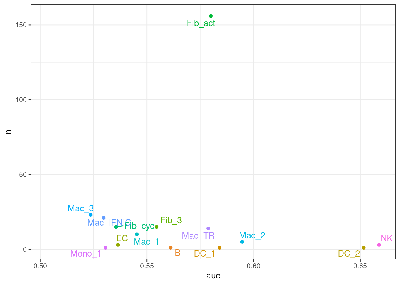
| Version | Author | Date |
|---|---|---|
| a71b19c | Florian Wuennemann | 2022-04-19 |
Looking at the AUC calculated by AUGUR and the number of differentially expressed genes, it seems like there is no correlation between the two measures.
sessionInfo()R version 4.1.3 (2022-03-10)
Platform: x86_64-pc-linux-gnu (64-bit)
Running under: Ubuntu 20.04.4 LTS
Matrix products: default
BLAS: /usr/lib/x86_64-linux-gnu/blas/libblas.so.3.9.0
LAPACK: /usr/lib/x86_64-linux-gnu/lapack/liblapack.so.3.9.0
locale:
[1] LC_CTYPE=en_US.UTF-8 LC_NUMERIC=C
[3] LC_TIME=de_DE.UTF-8 LC_COLLATE=en_US.UTF-8
[5] LC_MONETARY=de_DE.UTF-8 LC_MESSAGES=en_US.UTF-8
[7] LC_PAPER=de_DE.UTF-8 LC_NAME=C
[9] LC_ADDRESS=C LC_TELEPHONE=C
[11] LC_MEASUREMENT=de_DE.UTF-8 LC_IDENTIFICATION=C
attached base packages:
[1] stats graphics grDevices utils datasets methods base
other attached packages:
[1] here_1.0.1 ggrepel_0.9.1 scales_1.2.0 viridis_0.6.2
[5] viridisLite_0.4.0 Augur_1.0.3 cowplot_1.1.1 forcats_0.5.1
[9] stringr_1.4.0 dplyr_1.0.8 purrr_0.3.4 readr_2.1.2
[13] tidyr_1.2.0 tibble_3.1.6 ggplot2_3.3.5 tidyverse_1.3.1
[17] data.table_1.14.2 SeuratObject_4.0.4 Seurat_4.1.0 workflowr_1.7.0
loaded via a namespace (and not attached):
[1] utf8_1.2.2 R.utils_2.11.0 reticulate_1.24
[4] tidyselect_1.1.2 htmlwidgets_1.5.4 grid_4.1.3
[7] Rtsne_0.15 pROC_1.18.0 munsell_0.5.0
[10] codetools_0.2-18 ica_1.0-2 future_1.24.0
[13] miniUI_0.1.1.1 withr_2.5.0 tester_0.1.7
[16] spatstat.random_2.2-0 colorspace_2.0-3 highr_0.9
[19] knitr_1.38 rstudioapi_0.13 stats4_4.1.3
[22] ROCR_1.0-11 tensor_1.5 pbmcapply_1.5.0
[25] listenv_0.8.0 labeling_0.4.2 MatrixGenerics_1.7.0
[28] git2r_0.30.1 polyclip_1.10-0 farver_2.1.0
[31] rprojroot_2.0.3 parallelly_1.31.0 vctrs_0.4.1
[34] generics_0.1.2 ipred_0.9-12 xfun_0.30
[37] R6_2.5.1 rsvd_1.0.5 pals_1.7
[40] flexmix_2.3-17 spatstat.utils_2.3-0 assertthat_0.2.1
[43] promises_1.2.0.1 nnet_7.3-17 gtable_0.3.0
[46] globals_0.14.0 processx_3.5.3 goftest_1.2-3
[49] timeDate_3043.102 rlang_1.0.2 splines_4.1.3
[52] lazyeval_0.2.2 yardstick_0.0.9 dichromat_2.0-0
[55] spatstat.geom_2.4-0 broom_0.8.0 BiocManager_1.30.16
[58] yaml_2.3.5 reshape2_1.4.4 abind_1.4-5
[61] modelr_0.1.8 backports_1.4.1 httpuv_1.6.5
[64] tools_4.1.3 lava_1.6.10 ellipsis_0.3.2
[67] spatstat.core_2.4-2 jquerylib_0.1.4 RColorBrewer_1.1-3
[70] ggridges_0.5.3 Rcpp_1.0.8.3 parsnip_0.2.1
[73] plyr_1.8.7 sparseMatrixStats_1.7.0 ps_1.6.0
[76] rpart_4.1.16 deldir_1.0-6 pbapply_1.5-0
[79] zoo_1.8-9 haven_2.4.3 cluster_2.1.3
[82] fs_1.5.2 furrr_0.2.3 magrittr_2.0.3
[85] scattermore_0.8 lmtest_0.9-40 reprex_2.0.1
[88] RANN_2.6.1 whisker_0.4 fitdistrplus_1.1-8
[91] matrixStats_0.61.0 hms_1.1.1 patchwork_1.1.1
[94] mime_0.12 evaluate_0.15 xtable_1.8-4
[97] readxl_1.4.0 gridExtra_2.3 compiler_4.1.3
[100] maps_3.4.0 KernSmooth_2.23-20 crayon_1.5.1
[103] R.oo_1.24.0 htmltools_0.5.2 mgcv_1.8-40
[106] later_1.3.0 tzdb_0.3.0 lubridate_1.8.0
[109] DBI_1.1.2 dbplyr_2.1.1 MASS_7.3-56
[112] Matrix_1.4-1 cli_3.2.0 R.methodsS3_1.8.1
[115] parallel_4.1.3 gower_1.0.0 igraph_1.3.0
[118] pkgconfig_2.0.3 getPass_0.2-2 plotly_4.10.0
[121] spatstat.sparse_2.1-0 recipes_0.2.0 xml2_1.3.3
[124] bslib_0.3.1 hardhat_0.2.0 prodlim_2019.11.13
[127] rvest_1.0.2 callr_3.7.0 digest_0.6.29
[130] sctransform_0.3.3 RcppAnnoy_0.0.19 spatstat.data_2.1-4
[133] rmarkdown_2.13 cellranger_1.1.0 leiden_0.3.9
[136] uwot_0.1.11 modeltools_0.2-23 shiny_1.7.1
[139] lifecycle_1.0.1 nlme_3.1-157 jsonlite_1.8.0
[142] SeuratWrappers_0.3.0 mapproj_1.2.8 fansi_1.0.3
[145] pillar_1.7.0 lattice_0.20-45 fastmap_1.1.0
[148] httr_1.4.2 survival_3.2-13 remotes_2.4.2
[151] glue_1.6.2 png_0.1-7 class_7.3-20
[154] stringi_1.7.6 sass_0.4.1 rsample_0.1.1
[157] irlba_2.3.5 future.apply_1.8.1