6: Cell type abundance analysis
Florian Wuenenmann
3/16/2022
Last updated: 2022-04-19
Checks: 7 0
Knit directory: Abatacept_scrnaseq_mi/
This reproducible R Markdown analysis was created with workflowr (version 1.7.0). The Checks tab describes the reproducibility checks that were applied when the results were created. The Past versions tab lists the development history.
Great! Since the R Markdown file has been committed to the Git repository, you know the exact version of the code that produced these results.
Great job! The global environment was empty. Objects defined in the global environment can affect the analysis in your R Markdown file in unknown ways. For reproduciblity it’s best to always run the code in an empty environment.
The command set.seed(20220318) was run prior to running the code in the R Markdown file. Setting a seed ensures that any results that rely on randomness, e.g. subsampling or permutations, are reproducible.
Great job! Recording the operating system, R version, and package versions is critical for reproducibility.
Nice! There were no cached chunks for this analysis, so you can be confident that you successfully produced the results during this run.
Great job! Using relative paths to the files within your workflowr project makes it easier to run your code on other machines.
Great! You are using Git for version control. Tracking code development and connecting the code version to the results is critical for reproducibility.
The results in this page were generated with repository version 6fc473c. See the Past versions tab to see a history of the changes made to the R Markdown and HTML files.
Note that you need to be careful to ensure that all relevant files for the analysis have been committed to Git prior to generating the results (you can use wflow_publish or wflow_git_commit). workflowr only checks the R Markdown file, but you know if there are other scripts or data files that it depends on. Below is the status of the Git repository when the results were generated:
Ignored files:
    Ignored:    .Rhistory
    Ignored:    .Rproj.user/

Untracked files:
    Untracked:  code/utils.R
    Untracked:  code/utils_nichenet.R
    Untracked:  data/Table_1_Common Transcriptomic Effects of Abatacept and Other DMARDs on Rheumatoid Arthritis Synovial Tissue.xlsx
    Untracked:  omnipathr-log/

Unstaged changes:
    Deleted:    analysis/7_Conclusions.Rmd
    Deleted:    analysis/7_summary.Rmd
Note that any generated files, e.g. HTML, png, CSS, etc., are not included in this status report because it is ok for generated content to have uncommitted changes.
These are the previous versions of the repository in which changes were made to the R Markdown (analysis/6_differential_cell_type_abundance.Rmd) and HTML (docs/6_differential_cell_type_abundance.html) files. If you’ve configured a remote Git repository (see ?wflow_git_remote), click on the hyperlinks in the table below to view the files as they were in that past version.
| File | Version | Author | Date | Message |
|---|---|---|---|---|
| html | a71b19c | Florian Wuennemann | 2022-04-19 | Build site. |
| html | f472db4 | Florian Wuennemann | 2022-04-14 | Build site. |
| html | 6e3bb2f | Florian Wuennemann | 2022-03-25 | Build site. |
| html | 7eb9cc8 | Florian Wuennemann | 2022-03-25 | Build site. |
| Rmd | cb01216 | Florian Wuennemann | 2022-03-25 | wflow_publish("analysis/6_differential_cell_type_abundance.Rmd") |
| html | e38bb7b | Florian Wuennemann | 2022-03-24 | Build site. |
| Rmd | d5f28d4 | Florian Wuennemann | 2022-03-24 | wflow_publish("analysis/6_differential_cell_type_abundance.Rmd") |
| html | 46f2db7 | Florian Wuennemann | 2022-03-23 | First commit. |
Aim
In this markdown, we will use the package DASeq to try and identify differential abundant cells between control and Abatacept treated samples.
Load data
First we load our processed Seurat object.
seurat_object_filt <- readRDS("../data/2_annotated.seurat_object.rds")Prepare data
Then we will extract some metadata information that we need to run DASeq from the seurat object.
## Set sample labels
sample_treat_labels <- seurat_object_filt@meta.data %>%
  group_by(orig.ident,group) %>%
  select(orig.ident,group) %>%
  unique()

labels_control <- subset(sample_treat_labels,group == "control")$orig.ident
labels_treatment <- subset(sample_treat_labels,group == "treatment")$orig.ident
Run DASeq
No we will run DASeq to identify clusters in our data that show signs of differential abundance between control and treatment samples.
## Save DA object
da_object_name <- "../results/DA_object.rds"
if(file.exists(da_object_name)){
  da_cells <- readRDS(da_object_name)
}else{
  da_cells <- getDAcells(
    X = seurat_object_filt@reductions$pca@cell.embeddings[,1:20],
    cell.labels = seurat_object_filt@meta.data$orig.ident,
    labels.1 = labels_control,
    labels.2 = labels_treatment,
    k.vector = seq(50, 500, 50),
    plot.embedding = seurat_object_filt@reductions$umap@cell.embeddings)
  saveRDS(da_cells,
          file = da_object_name)
}

da_cells$da.cells.plot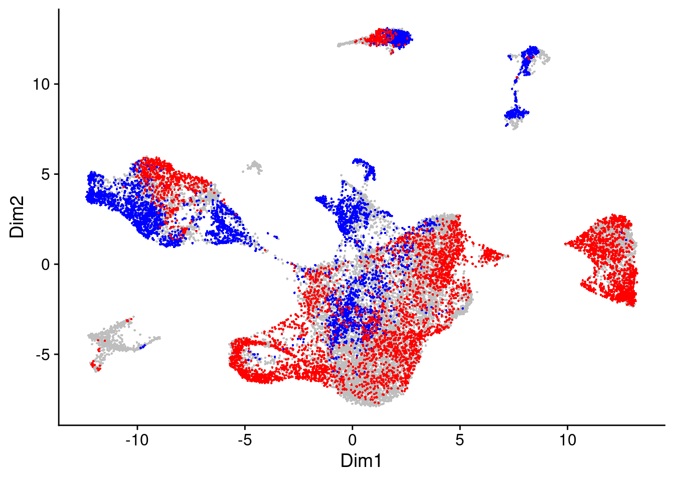
| Version | Author | Date |
|---|---|---|
| 7eb9cc8 | Florian Wuennemann | 2022-03-25 |
We will take a look at the randplot that gives a measure of the distribution of DA cell scores created by permutation. The lightgrey curve here represents the distribution of DA measure scores from the permutation analysis. By default, cells with scores that fall outside that distribution are selected as DA cells.
##
da_cells$rand.plot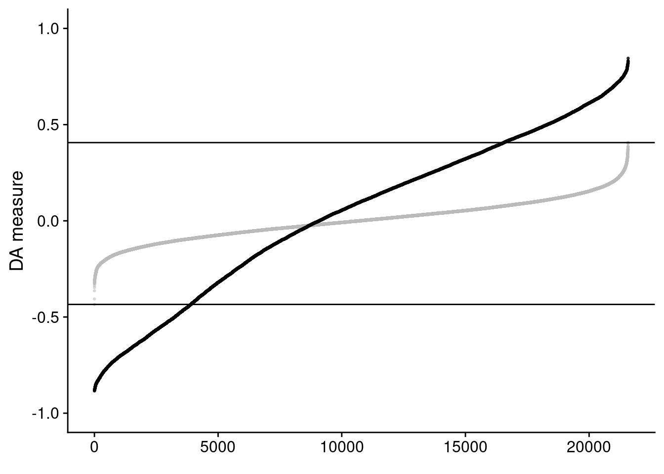
| Version | Author | Date |
|---|---|---|
| 7eb9cc8 | Florian Wuennemann | 2022-03-25 |
Since this is a pretty relaxed filtering threshold, let’s be a bit more strict and increase this DA measure threshold a bit.
da_cells <- updateDAcells(
  X = da_cells,
  pred.thres = c(-0.75,0.75),
  plot.embedding = seurat_object_filt@reductions$umap@cell.embeddings
)
da_cells$da.cells.plot
Now we can use the DA cells to cluster them into DA regions, i.e. regions with differential abundance from the two treatment groups.
da_regions <- getDAregion(
  X = seurat_object_filt@reductions$pca@cell.embeddings[,1:20],
  da.cells = da_cells,
  cell.labels = seurat_object_filt@meta.data$orig.ident,
  labels.1 = labels_control,
  labels.2 = labels_treatment,
  resolution = 0.01,
  plot.embedding = seurat_object_filt@reductions$umap@cell.embeddings,
  min.cell = 20
)
Warning: Feature names cannot have underscores ('_'), replacing with dashes
('-')
Warning: Feature names cannot have underscores ('_'), replacing with dashes
('-')
Warning: Feature names cannot have underscores ('_'), replacing with dashes
('-')Removing 10 DA regions with cells < 20.Warning in wilcox.test.default(x = idx.label.ratio[labels.2],
idx.label.ratio[labels.1]): cannot compute exact p-value with tiesNow let’s visualize a number of different features on top of these plots. First, let’s check cell types, then the treatment group, followed by the DA score and then the DA subclusters.
## Plot different measures on top of the UMAP
DimPlot(seurat_object_filt,reduction = "umap", label = TRUE) ## UMAP with cellt types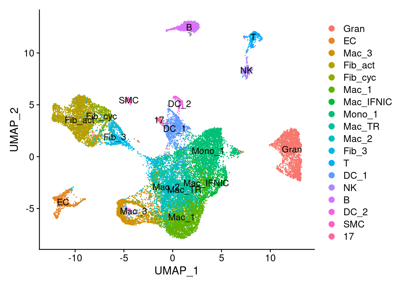
| Version | Author | Date |
|---|---|---|
| 7eb9cc8 | Florian Wuennemann | 2022-03-25 |
DimPlot(seurat_object_filt, group.by = "group") ## UMAP with treatment group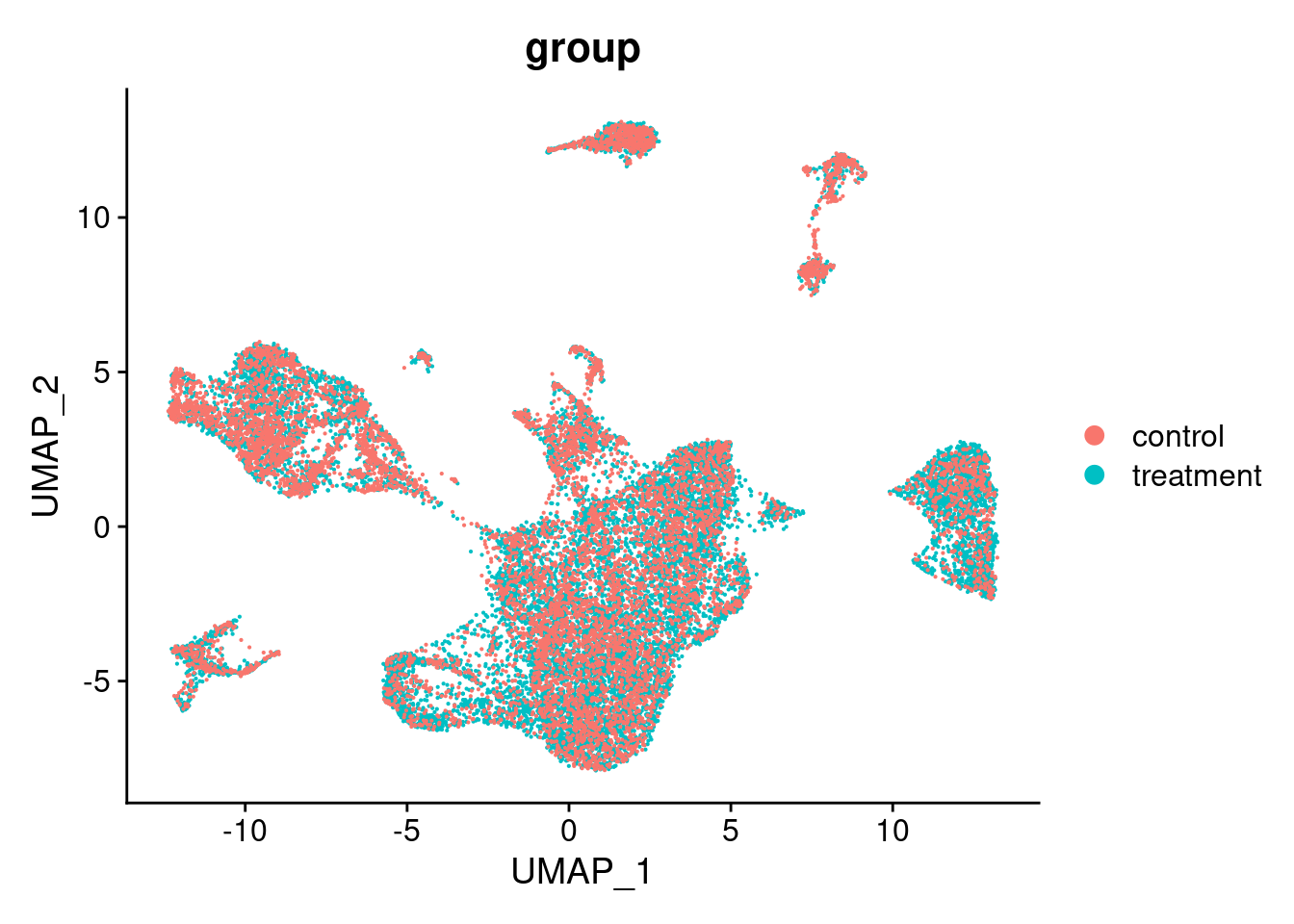
| Version | Author | Date |
|---|---|---|
| 7eb9cc8 | Florian Wuennemann | 2022-03-25 |
da_cells$da.cells.plot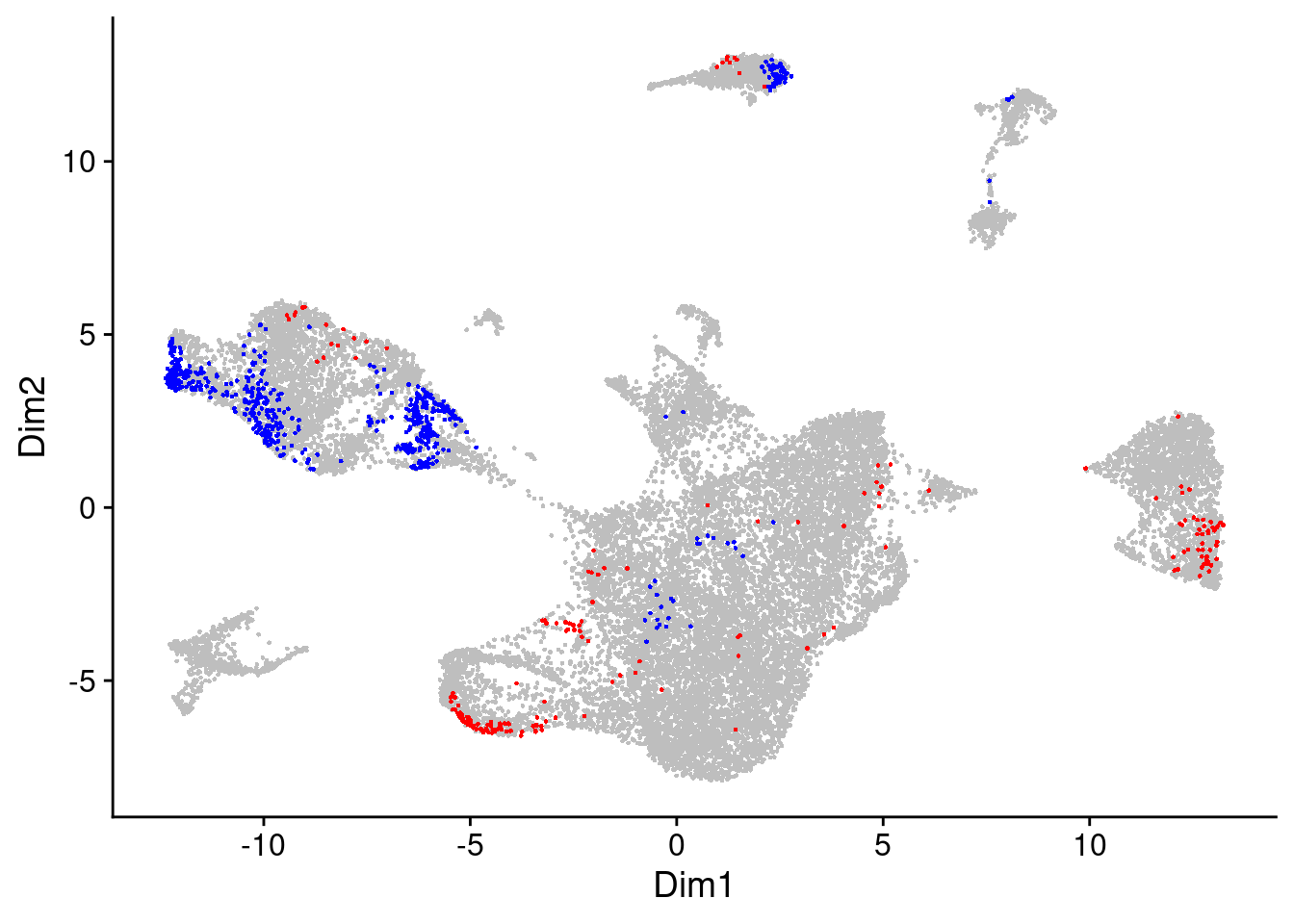
| Version | Author | Date |
|---|---|---|
| 7eb9cc8 | Florian Wuennemann | 2022-03-25 |
da_regions$da.region.plot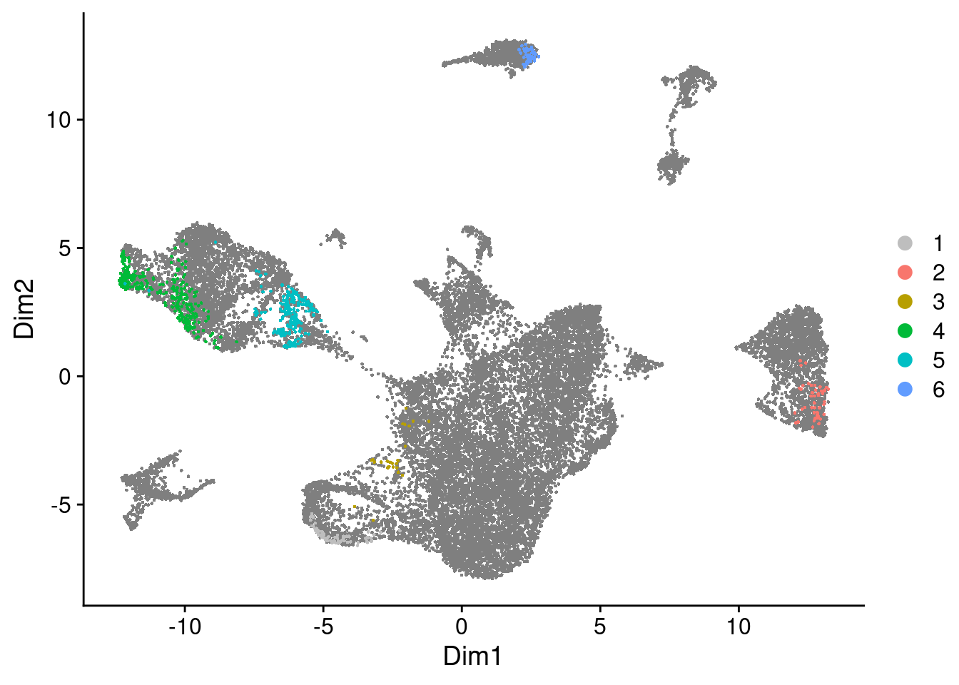
| Version | Author | Date |
|---|---|---|
| 7eb9cc8 | Florian Wuennemann | 2022-03-25 |
Now we can also identify genes that classify these subclusters of differentially abundant cells.
## Lets use the SeuratMarkerFinder function from DASeq to find
## Add DA regions to seruat metadata
seurat_object_filt$da <- da_regions$da.region.label
da_scores <- da_regions$DA.stat
all_da_markers <- data.frame()
## Save STG gene set
all_marker_object_name <- "../results/DA_analysis.STG_genes.rds"
if(file.exists(all_marker_object_name)){
all_da_markers <- readRDS(all_marker_object_name)
}else{
for(this_celltype in unique(seurat_object_filt$cell_type)){
print(this_celltype)
seurat_subset <- subset(seurat_object_filt,cell_type == this_celltype)
n_da_region <- length(unique(seurat_subset$da))
if(n_da_region > 1 & nrow(subset(seurat_subset@meta.data,da !=0)) > 10){
da_numbers <- setdiff(unique(seurat_subset$da),c(0))
for(da_region in da_numbers){
print(da_region)
da_score <- da_scores[as.numeric(da_region),]
if(da_score[1] > 0){
direction <- "higher_in_treatment"
}else{
direction <- "higher_in_control"
}
da_markers <- FindMarkers(object = seurat_subset,
group.by = "da",
ident.1 = da_region,
ident.2 = 0)
da_markers$da_region <- da_region
da_markers$celltype_cluster <- this_celltype
da_markers$feature <- rownames(da_markers)
da_markers <- da_markers %>%
mutate("DA_direction" = direction)
all_da_markers <- rbind(all_da_markers,da_markers)
}
}
}
saveRDS(all_da_markers,
file = all_marker_object_name)
}
all_da_markers_sig <- all_da_markers %>%
subset(p_val_adj < 0.05) %>%
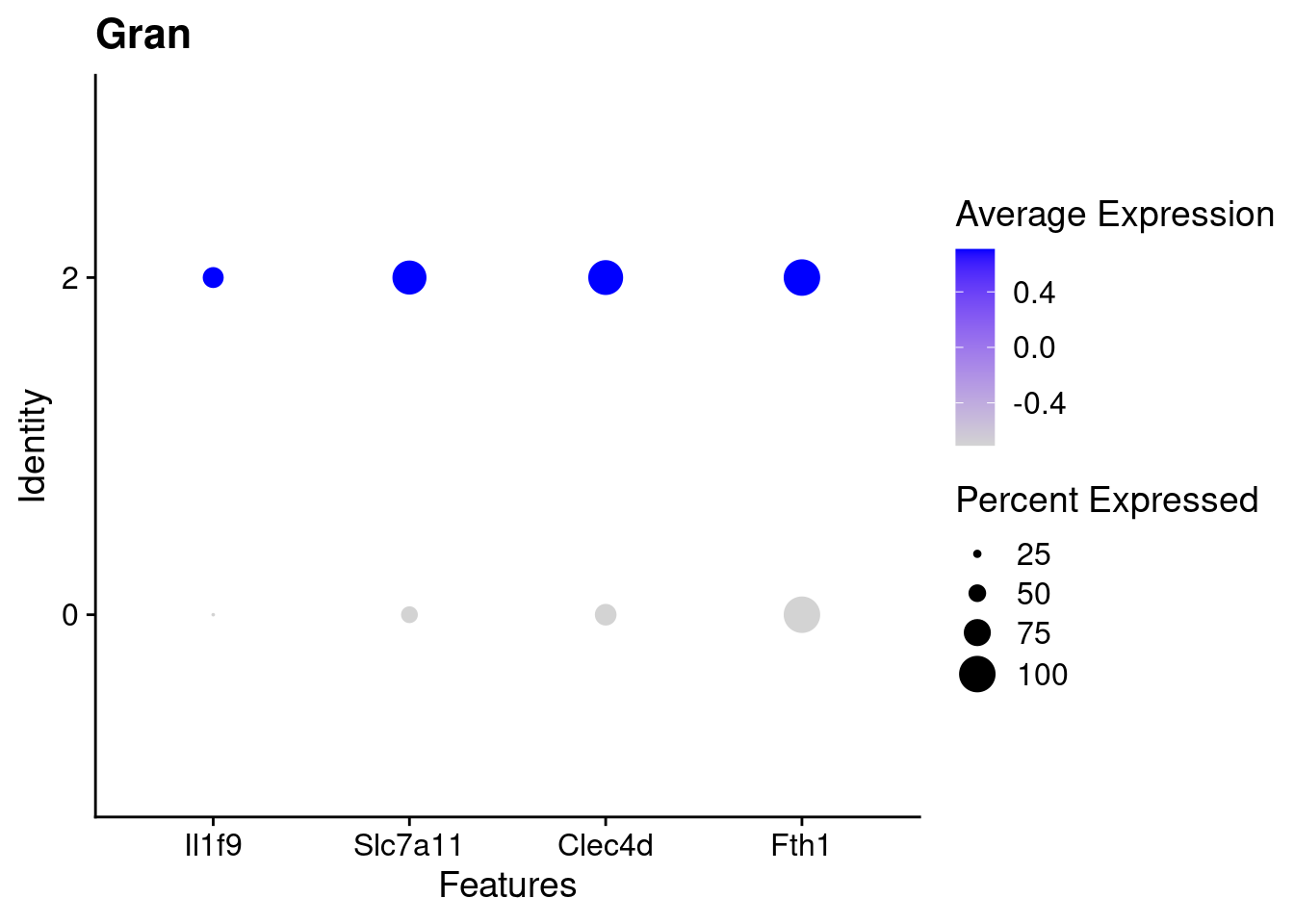
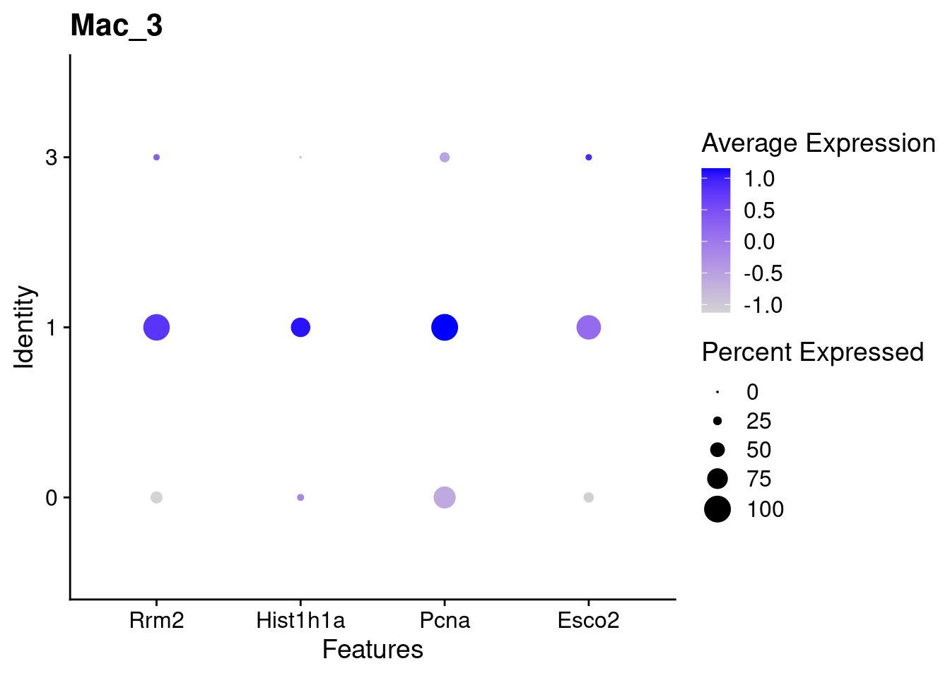
arrange(p_val_adj)Plot DA region markers
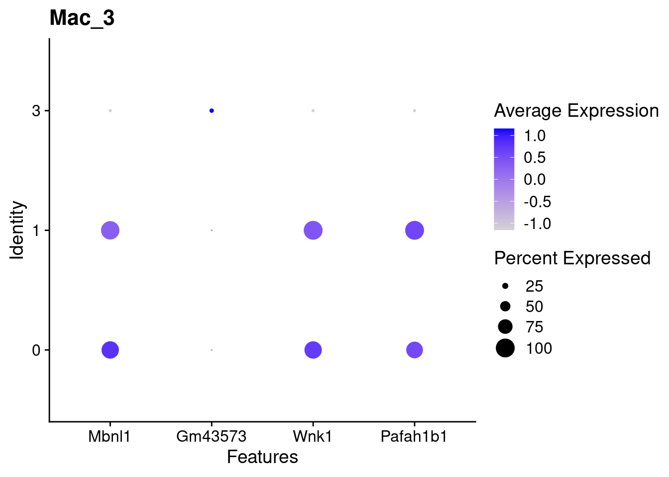
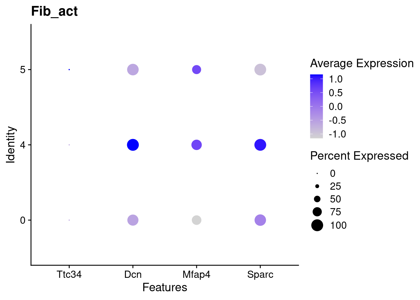
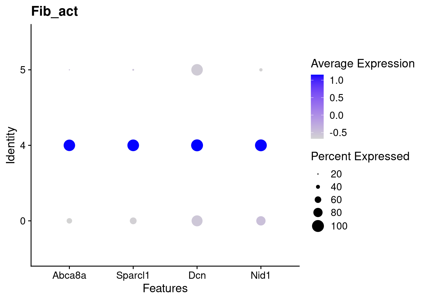
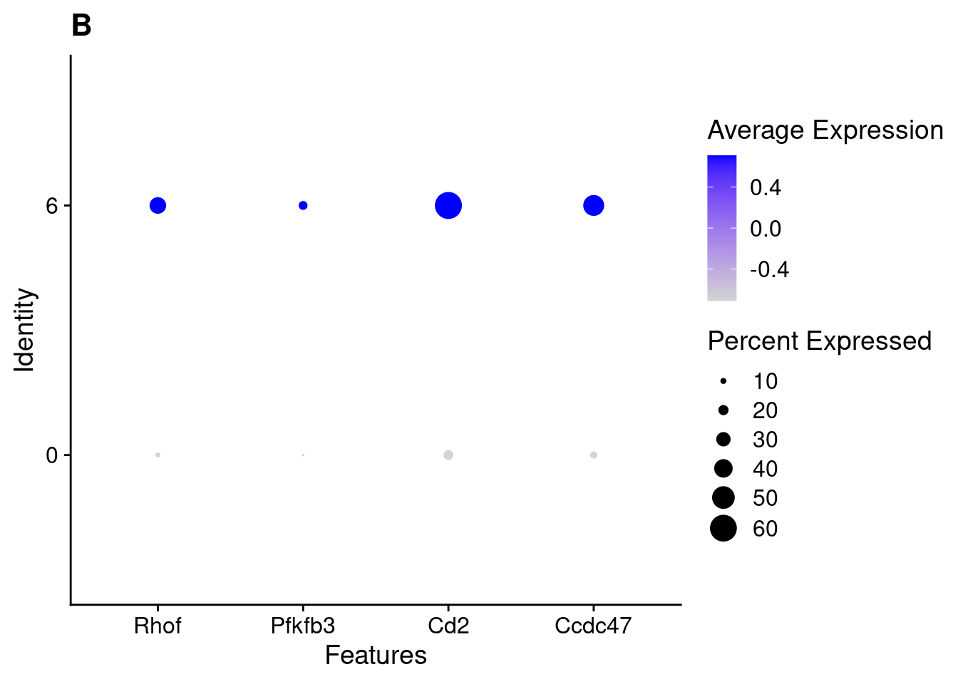
for(this_daregion in unique(all_da_markers$da_region)){
  ## Plot Dotplot similar to original DASeq publication
  da_markers <- subset(all_da_markers,da_region == this_daregion)
  this_celltype <- unique(da_markers$celltype_cluster)
  seurat_subset <- subset(seurat_object_filt,cell_type == this_celltype)
  top_markers <- da_markers %>%
    top_n(4,wt = - p_val_adj)

  dotplot <- DotPlot(seurat_subset,
                     features = top_markers$feature,
                     group.by = "da") +
    labs(title = this_celltype)

  print(dotplot)
}
| Version | Author | Date |
|---|---|---|
| 7eb9cc8 | Florian Wuennemann | 2022-03-25 |
| Version | Author | Date |
|---|---|---|
| 7eb9cc8 | Florian Wuennemann | 2022-03-25 |
reactable(all_da_markers_sig,
          resizable = TRUE, showPageSizeOptions = TRUE,
          searchable = TRUE,filterable = TRUE,
          onClick = "expand", highlight = TRUE)
Conclusion
Using DASeq, we were able to identify several different regions of differentiall abundant (DA) cells for different subtypes of cells. From a quick cross-check, it looks like this analysis is in line with the initial finding of higher immune cells in Abatacept treated samples and higher fibroblast cell content in control samples.
sessionInfo()R version 4.1.3 (2022-03-10)
Platform: x86_64-pc-linux-gnu (64-bit)
Running under: Ubuntu 20.04.4 LTS
Matrix products: default
BLAS: /usr/lib/x86_64-linux-gnu/blas/libblas.so.3.9.0
LAPACK: /usr/lib/x86_64-linux-gnu/lapack/liblapack.so.3.9.0
locale:
[1] LC_CTYPE=en_US.UTF-8 LC_NUMERIC=C
[3] LC_TIME=de_DE.UTF-8 LC_COLLATE=en_US.UTF-8
[5] LC_MONETARY=de_DE.UTF-8 LC_MESSAGES=en_US.UTF-8
[7] LC_PAPER=de_DE.UTF-8 LC_NAME=C
[9] LC_ADDRESS=C LC_TELEPHONE=C
[11] LC_MEASUREMENT=de_DE.UTF-8 LC_IDENTIFICATION=C
attached base packages:
[1] stats graphics grDevices utils datasets methods base
other attached packages:
[1] reactable_0.2.3 data.table_1.14.2 DAseq_1.0.0 forcats_0.5.1
[5] stringr_1.4.0 dplyr_1.0.8 purrr_0.3.4 readr_2.1.2
[9] tidyr_1.2.0 tibble_3.1.6 ggplot2_3.3.5 tidyverse_1.3.1
[13] SeuratObject_4.0.4 Seurat_4.1.0 workflowr_1.7.0
loaded via a namespace (and not attached):
[1] utf8_1.2.2 reticulate_1.24 R.utils_2.11.0
[4] tidyselect_1.1.2 htmlwidgets_1.5.4 grid_4.1.3
[7] Rtsne_0.15 pROC_1.18.0 munsell_0.5.0
[10] codetools_0.2-18 ica_1.0-2 future_1.24.0
[13] miniUI_0.1.1.1 withr_2.5.0 spatstat.random_2.2-0
[16] colorspace_2.0-3 highr_0.9 knitr_1.38
[19] rstudioapi_0.13 stats4_4.1.3 ROCR_1.0-11
[22] tensor_1.5 listenv_0.8.0 labeling_0.4.2
[25] git2r_0.30.1 polyclip_1.10-0 farver_2.1.0
[28] rprojroot_2.0.3 parallelly_1.31.0 vctrs_0.4.1
[31] generics_0.1.2 ipred_0.9-12 xfun_0.30
[34] R6_2.5.1 rsvd_1.0.5 flexmix_2.3-17
[37] spatstat.utils_2.3-0 assertthat_0.2.1 promises_1.2.0.1
[40] scales_1.2.0 nnet_7.3-17 gtable_0.3.0
[43] globals_0.14.0 processx_3.5.3 goftest_1.2-3
[46] timeDate_3043.102 rlang_1.0.2 splines_4.1.3
[49] lazyeval_0.2.2 ModelMetrics_1.2.2.2 spatstat.geom_2.4-0
[52] broom_0.8.0 BiocManager_1.30.16 yaml_2.3.5
[55] reshape2_1.4.4 abind_1.4-5 modelr_0.1.8
[58] crosstalk_1.2.0 backports_1.4.1 httpuv_1.6.5
[61] caret_6.0-91 tools_4.1.3 lava_1.6.10
[64] ellipsis_0.3.2 spatstat.core_2.4-2 jquerylib_0.1.4
[67] RColorBrewer_1.1-3 proxy_0.4-26 ggridges_0.5.3
[70] Rcpp_1.0.8.3 plyr_1.8.7 ps_1.6.0
[73] rpart_4.1.16 deldir_1.0-6 pbapply_1.5-0
[76] cowplot_1.1.1 zoo_1.8-9 reactR_0.4.4
[79] haven_2.4.3 ggrepel_0.9.1 cluster_2.1.3
[82] fs_1.5.2 magrittr_2.0.3 scattermore_0.8
[85] lmtest_0.9-40 reprex_2.0.1 RANN_2.6.1
[88] whisker_0.4 fitdistrplus_1.1-8 matrixStats_0.61.0
[91] hms_1.1.1 patchwork_1.1.1 mime_0.12
[94] evaluate_0.15 xtable_1.8-4 readxl_1.4.0
[97] gridExtra_2.3 shape_1.4.6 compiler_4.1.3
[100] KernSmooth_2.23-20 crayon_1.5.1 R.oo_1.24.0
[103] htmltools_0.5.2 mgcv_1.8-40 later_1.3.0
[106] tzdb_0.3.0 lubridate_1.8.0 DBI_1.1.2
[109] dbplyr_2.1.1 MASS_7.3-56 Matrix_1.4-1
[112] cli_3.2.0 R.methodsS3_1.8.1 parallel_4.1.3
[115] gower_1.0.0 igraph_1.3.0 pkgconfig_2.0.3
[118] getPass_0.2-2 plotly_4.10.0 spatstat.sparse_2.1-0
[121] recipes_0.2.0 xml2_1.3.3 foreach_1.5.2
[124] bslib_0.3.1 hardhat_0.2.0 prodlim_2019.11.13
[127] rvest_1.0.2 callr_3.7.0 digest_0.6.29
[130] sctransform_0.3.3 RcppAnnoy_0.0.19 spatstat.data_2.1-4
[133] rmarkdown_2.13 cellranger_1.1.0 leiden_0.3.9
[136] uwot_0.1.11 modeltools_0.2-23 shiny_1.7.1
[139] lifecycle_1.0.1 nlme_3.1-157 jsonlite_1.8.0
[142] SeuratWrappers_0.3.0 viridisLite_0.4.0 fansi_1.0.3
[145] pillar_1.7.0 lattice_0.20-45 fastmap_1.1.0
[148] httr_1.4.2 survival_3.2-13 glue_1.6.2
[151] remotes_2.4.2 png_0.1-7 iterators_1.0.14
[154] glmnet_4.1-3 class_7.3-20 stringi_1.7.6
[157] sass_0.4.1 irlba_2.3.5 e1071_1.7-9
[160] future.apply_1.8.1